- Design of five types of seismic force-resisting systems (SFRS) includes Special Moment Frame (SMF), Intermediate Moment Frame (IMF), Ordinary Moment Frame (OMF), Ordinary Concentrically Braced Frame (OCBF), and Special Concentrically Braced Frame (SCBF)
- Ductility check of the width-to thickness ratios for webs and flanges
- Calculation of the required strength and stiffness for stability bracing of beams
- Calculation of the maximum spacing for stability bracing of beams
- Calculation of the required strength at hinge locations for stability bracing of beams
- Calculation of the column required strength with the option to neglect all bending moments, shear, and torsion for overstrength limit state
- Design check of column and brace slenderness ratios
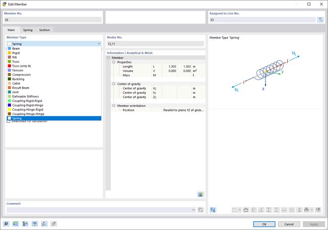
The "Spring" member type is used to simulate linear and nonlinear spring properties via a linear object. This input function helps you to model the stiffness specifications in the force/displacement unit.
Go to Explanatory Video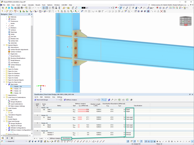
In the Steel Joints add-on, you can classify the joint stiffness.
In addition to the initial stiffness, the table also shows the limit values for hinged and rigid connections for the selected internal forces N, My, and/or Mz. The resulting classification is then displayed in tables as "hinged", "semi-rigid", or "rigid".
Go to Explanatory Video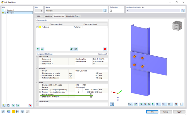
In the Steel Joints add-on, you have this option to consider the preloaded bolts in the calculation of all components.
You can easily activate the prestress using the check box in the bolt parameters, and it has an impact on the stress-strain analysis as well as the stiffness analysis.
Go to Explanatory Video
Using the "Load Transfer Only" story type, you can consider slabs without stiffness effect in and out of the plane in the Building Model add-on. This element type collects the loads on the slab and transfers them to the supporting elements of a 3D model. Thus, you can simulate secondary components, such as grillage and similar load distribution elements, without any further effect in the 3D model.
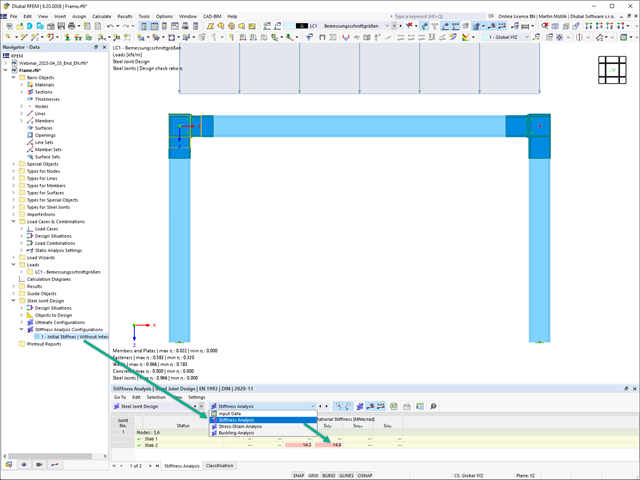
In the Steel Joints add-on, you can determine the initial stiffness Sj,ini according to Eurocode and AISC. This can be done for selected members with reference to the internal forces N, My, and Mz.
In the Members tab of the input dialog box of the Steel Joints add-on, you can select the desired internal forces via a checkbox. Multiple selection is possible. For these internal forces, the stiffness analysis is carried out with a positive and a negative sign.
Go to Explanatory Video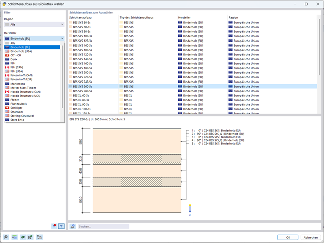
A library for cross-laminated timber panels is implemented in RFEM, from which you can import the manufacturer's layer structures (for example, Binderholz, KLH, Piveteaubois, Södra, Züblin Timber, Schilliger, Stora Enso). In addition to the layer thicknesses and materials, there is also the information about stiffness reductions and the narrow side bonding.
Go to Explanatory Video
When defining the input data for the modal analysis load case, you can consider a load case whose stiffnesses represent the initial position for the modal analysis. How do you do that? As shown in the image, select the "Consider initial state from" option. Now, open the "Initial State Settings" dialog box and define the type Stiffness as the initial state. In this load case, as of which is the initial state taken into account, you can consider the stiffness of the structural system when the tension members fail. The purpose of all of this: The stiffness from this load case is considered in the modal analysis. Thus, you obtain a clearly flexible system.

Did you know? You can easily define structural modifications in load cases of the Modal Analysis type. This allows you, for example, to individually adjust the stiffnesses of materials, cross-sections, members, surfaces, hinges, and supports. You can also modify stiffnesses for some design add-ons. Once you select the objects, their stiffness properties are adapted to the object type. In this way, you can define them in separate tabs.
Do you want to analyze the failure of an object (for example, a column) in the modal analysis? This is also possible without any problems. Simply switch to the Structure Modification window and deactivate the relevant objects.

RFEM allows you to use a special line hinge to model the special properties of the connection between the reinforced concrete slab and masonry wall. This limits the transferable forces of the connection depending on the specified geometry. You guess right: This means that the material cannot be overloaded.
The program develops interaction diagrams that are applied automatically. They represent the various geometric situations and you can use them to determine the correct stiffness.
- Stability analyses for flexural buckling, torsional buckling, and flexural-torsional buckling under compression
- Import of the effective lengths from the calculation using the Structure Stability add-on
- Graphical input and check of the defined nodal supports and effective lengths for stability analysis
- Determination of the equivalent member lengths for tapered members
- Consideration of Lateral-Torsional Bracing Position
- Lateral-torsional buckling analysis of the structural components subjected to moment loading
- Depending on the standard, a choice between user-defined input of Mcr, analytical method from the standard, and use of internal eigenvalue solver
- Consideration of a shear panel and a rotational restraint when using the eigenvalue solver
- Graphical display of a mode shape if the eigenvalue solver was used
- Stability analysis of structural components with the combined compression and bending stress, depending on the design standard
- Comprehensible calculation of all necessary coefficients, such as the factors for considering moment distribution or interaction factors
- Alternative consideration of all effects for the stability analysis when determining internal forces in RFEM/RSTAB (second-order analysis, imperfections, stiffness reduction, possibly in combination with the Torsional Warping (7 DOF) add-on)
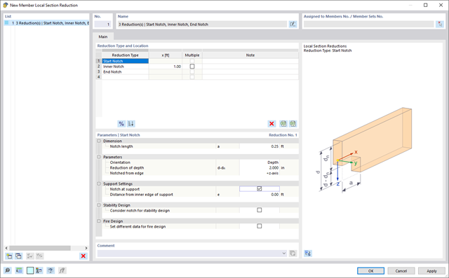
Use the member cross-section reductions to consider the start, internal, or end notches of a beam. The beam reduction is thus taken into account in the calculation of the load-bearing capacity. However, this does not apply to the stiffness.
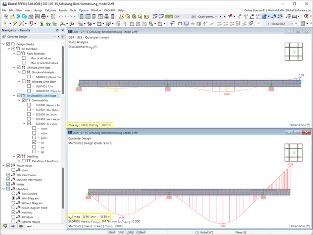
- Calculation of deflections and comparison with the normative or manually adjusted limit values
- Consideration of a precamber for the deflection analysis
- Different limit values are possible, depending on the design situation type
- Manual adjustment of reference lengths and segmentation by direction
- Calculation of deflections related to the initial structure or to the deformed structure
- Automatic consideration of time-dependent deformations by increasing the load with the creep factor (can also be user-defined on the stiffness side)
- Simplified vibration design
- Graphical result display integrated in RFEM/RSTAB; for example, the design ratio of a limit value, the deformation, or the sag
- Complete integration of the results into the RFEM/RSTAB printout report
.png?mw=640&hash=342149908caead326e60e26a2b5d05f7f46825cb)
Are you familiar with the Tsai-Wu material model? It combines plastic and orthotropic properties, which allows for special modeling of materials with anisotropic characteristics, such as fiber-reinforced plastics or timber.
If the material is plastified, the stresses remain constant. The redistribution is carried out according to the stiffnesses available in the individual directions. The elastic area corresponds to the Orthotropic | Linear Elastic (Solids) material model. For the plastic area, the yielding according to Tsai-Wu applies:
All strengths are defined positively. You can imagine the stress criterion as an elliptical surface within a six-dimensional space of stresses. If one of the three stress components is applied as a constant value, the surface can be projected onto a three-dimensional stress space.
If the value for fy(σ), according to the Tsai-Wu equation, plane stress condition, is smaller than 1, the stresses are in the elastic zone. The plastic area is reached as soon as fy (σ) = 1; values greater than 1 are not allowed. The model behavior is ideal-plastic, which means there is no stiffening.

Did you know? In contrast to other material models, the stress-strain diagram for this material model is not antimetric to the origin. You can use this material model to simulate the behavior of steel fiber-reinforced concrete, for example. Find detailed information about modeling steel fiber-reinforced concrete in the technical article about Determining the material properties of steel-fiber-reinforced concrete.
In this material model, the isotropic stiffness is reduced with a scalar damage parameter. This damage parameter is determined from the stress curve defined in the Diagram. The direction of the principal stresses is not taken into account. Rather, the damage occurs in the direction of the equivalent strain, which also covers the third direction perpendicular to the plane. The tension and compression area of the stress tensor is treated separately. In this case, different damage parameters apply.
The "Reference element size" controls how the strain in the crack area is scaled to the length of the element. With the default value zero, no scaling is performed. Thus, the material behavior of the steel fiber concrete is modeled realistically.
Find more information about the theoretical background of the "Isotropic Damage" material model in the technical article describing the Nonlinear Material Model Damage.
You determine the deformation for members and surfaces, taking into account the cracked (state II) or non-cracked (state I) reinforced concrete cross-section. When determining the stiffness, you can consider "tension stiffening" between the cracks according to the design standard used.
.png?mw=640&hash=5a991f211d984ac624978f514e70c53da263e5d9)
Depending on the axial force N, you can generate a moment curvature line for any moment vector. The program also shows you the value pairs of the displayed diagram in a table. Furthermore, you can activate the secant stiffness and tangent stiffness of the reinforced concrete cross-section, belonging to the moment curvature diagram, as an additional diagram.
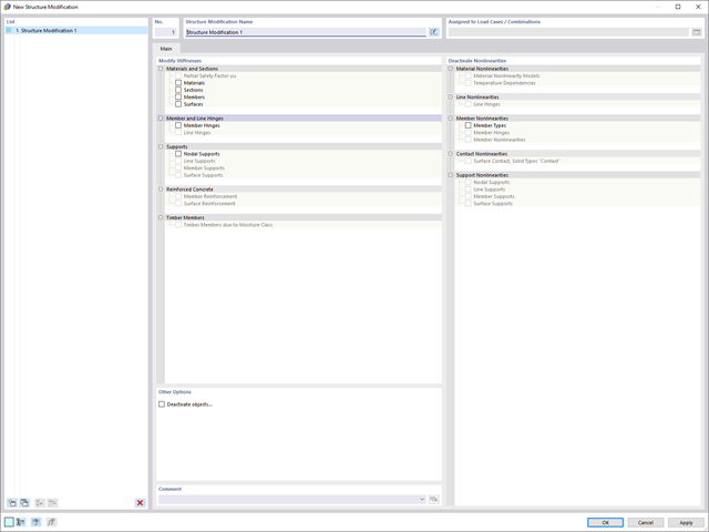
Use the new useful structure modification object to modify or deactivate stiffnesses, nonlinearities, and objects in a clear and load case-dependent way.
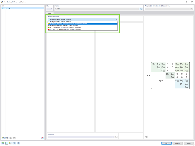
Do you want to modify surface stiffnesses? There are now two new types available for you:
- Multiplication factor of total stiffness
- Multiplication factors of partial stiffnesses, weights, and masses

Are you afraid that your project will end in the digital tower of Babel? The Building Model add-on for RFEM supports you in your work on a construction project with several stories. It allows you to define a building by means of stories at specified elevations. You can adjust the stories in many ways afterwards and also select the story slab stiffness. Information about the stories and the entire model (center of gravity, center of rigidity) is displayed for you in tables and graphics.
More About Building Model
Use the specification of the element types for members, surfaces, solids, and so on, to facilitate your input (such as member nonlinearities, member stiffnesses, design supports, and many others).
Keep an eye on all surfaces. A surface with the "Load Transfer" stiffness type has no structural effect. You can use it to consider the loads from surfaces that have not been modeled, for example, facade structures, glass surfaces, trapezoidal roof sections, and so on.
Go to Explanatory Video
Also in this case, RSTAB will certainly convince you. With the powerful calculation kernel, its optimized networking and support of multi-core processor technology, the Dlubal structural analysis program is far ahead. This allows you to calculate more linear load cases and load combinations using several processors in parallel without using additional memory. The stiffness matrix only has to be created once. Thus, it is possible for you to calculate even large systems with the fast and direct solver.
Do you have to calculate multiple load combinations in your models? The program initiates several solvers in parallel (one per core). Each solver then calculates a load combination for you. This leads to better utilization of the cores.
You can systematically follow the development of the deformation displayed in a diagram during the calculation, and thus precisely evaluate the convergence behavior.
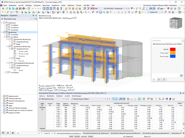
The Concrete Design add-on combines all CONCRETE add-on modules from RFEM 5 / RSTAB 8. Compared to these add-on modules, the following new features have been added to the Concrete Design add-on for RFEM 6 / RSTAB 9:
- Input of design-relevant specifications (effective lengths, durability, reinforcement directions, surface reinforcement) directly in the RFEM or RSTAB model
- Extensive input options for longitudinal and transverse reinforcement of members
- Detailed intermediate results for the design with specification of the equations of the applied standard for better traceability of the calculation
- New interaction diagram with interactive graphic for N, M, and M + N from cross-section design incl. output of the secant and tangent stiffness
- Design of the defined reinforcement in the ultimate limit state and serviceability limit state incl. graphical output of the design ratio for the respective component
- Automatic check of the defined reinforcement with regard to the construction or general reinforcement rules for reinforced member and surface components
- Cross-section design optionally with net values of the concrete section
- Design according to the Russian standard SP 63.13330

Compared to the RF-/STEEL Warping Torsion add-on module (RFEM 5 / RSTAB 8), the following new features have been added to the Torsional Warping (7 DOF) add-on for RFEM 6 / RSTAB 9:
- Complete integration into the environment of RFEM 6 and RSTAB 9
- 7th degree of freedom is directly taken into account in the calculation of members in RFEM/RSTAB on the entire system
- No more need to define support conditions or spring stiffnesses for calculation on the simplified equivalent system
- Combination with other add-ons is possible, for example for the calculation of critical loads for torsional buckling and lateral-torsional buckling with stability analysis
- No restriction to thin-walled steel sections (it is also possible to calculate ideal overturning moments for beams with massive timber sections, for example)

- Stress determination using an elastic-plastic material model
- Design of masonry disc structures for compression and shear on the building model or single model
- Automatic determination of stiffness of a wall-slab hinge
- An extensive material database for almost all stone-mortar combinations available on the Austrian market (the product range is continuously being expanded, for other countries as well)
- Automatic determination of material values according to Eurocode 6 (ÖN EN 1996‑X)
- Option to create pushover analysis

- Automatic consideration of masses from self-weight
- Direct import of masses from load cases or load combinations
- Optional definition of additional masses (nodal, linear, or surface masses, as well as inertia masses) directly in the load cases
- Optional neglect of masses (for example, mass of foundations)
- Combination of masses in different load cases and load combinations
- Preset combination coefficients for various standards (EC 8, SIA 261, ASCE 7,...)
- Optional import of initial states (for example, to consider prestress and imperfection)
- Structure Modification
- Consideration of failed supports or members/surfaces/solids
- Definition of several modal analyses (for example, to analyze different masses or stiffness modifications)
- Selection of mass matrix type (diagonal matrix, consistent matrix, unit matrix), including user-defined specification of translational and rotational degrees of freedom
- Methods for determining the number of mode shapes (user-defined, automatic - to reach effective modal mass factors, automatic - to reach the maximum natural frequency - only available in RSTAB)
- Determination of mode shapes and masses in nodes or FE mesh points
- Results of eigenvalue, angular frequency, natural frequency, and period
- Output of modal masses, effective modal masses, modal mass factors, and participation factors
- Masses in mesh points displayed in tables and graphics
- Visualization and animation of mode shapes
- Various scaling options for mode shapes
- Documentation of numerical and graphical results in printout report

In the modal analysis settings, you have to enter all data that are necessary for the determination of the natural frequencies. These are, for example, mass shapes and eigenvalue solvers.
The Modal Analysis add-on determines the lowest eigenvalues of the structure. Either you adjust the number of eigenvalues or let them determined automatically. Thus, you should reach either effective modal mass factors or maximum natural frequencies. Masses are imported directly from load cases and load combinations. In this case, you have the option to consider the total mass, load components in the global Z-direction, or only the load component in the direction of gravity.
You can manually define additional masses at nodes, lines, members, or surfaces. Furthermore, you can influence the stiffness matrix by importing axial forces or stiffness modifications of a load case or load combination.

- Consideration and display of story masses
- Listing of structural elements and their information
- Automated creation of result sections on shear walls
- Output of section resultants in global direction for determining shear forces
- Optional definition of rigid diaphragm by story (story modeling)
- Stiffness type Floor Slab - Rigid Diaphragm
- Defining floor sets,
- for example, calculation of slabs as a 2D position within the 3D model
- Shear walls: Automatic definition of result members with any cross-section
- Design of rectangular cross-sections using the Concrete Design add-on
- Definition of deep beams, design possible using the Concrete Design add-on
- Tabular output of story actions, interstory drift, and center points of mass and stiffness, as well as the forces in shear walls
- Separate result display of the floor and stiffening design
The standards already specify the approximation methods (for example, deformation calculation according to EN 1992‑1‑1, 7.4.3, or ACI 318‑19, 24.3.2.5) that you need for your deformation calculation. In this case, the so-called effective stiffnesses are calculated in the finite elements in accordance with the existing limit state with / without cracks. You can then use these effective stiffnesses to determine the deformations by means of another FEM calculation.
Consider a reinforced concrete cross-section for the calculation of the effective stiffnesses of the finite elements. Based on the internal forces determined for the serviceability limit state in RFEM, you can classify the reinforced concrete cross-section as "cracked" or "uncracked". Do you consider the effect of the concrete between the cracks? In this case, this is done by means of a distribution coefficient (for example, according to EN 1992‑1‑1, Eq. 7.19, or ACI 318‑19, 24.3.2.5). You can assume the material behavior for the concrete to be linear-elastic in the compression and tension zone until reaching the concrete tensile strength. This procedure is sufficiently precise for the serviceability limit state.
When determining the effective stiffnesses, you can take into accout the creep and shrinkage at the "cross-section level." You don't need to consider the influence of shrinkage and creep in statically indeterminate systems in this approximation method (for example, tensile forces from shrinkage strain in systems restrained on all sides are not determined and have to be considered separately). In summary, the deformation calculation is carried out in two steps:
- Calculation of effective stiffnesses of the reinforced concrete cross-section assuming linear-elastic conditions
- Calculation of the deformation using the effective stiffnesses with FEM