22 Wyniki
Wyświetl wyniki:
Sortuj według:
- 002074
- Ogólne informacje
- Analiza stateczności konstrukcji RFEM 6
- Analiza stateczności konstrukcji RSTAB 9
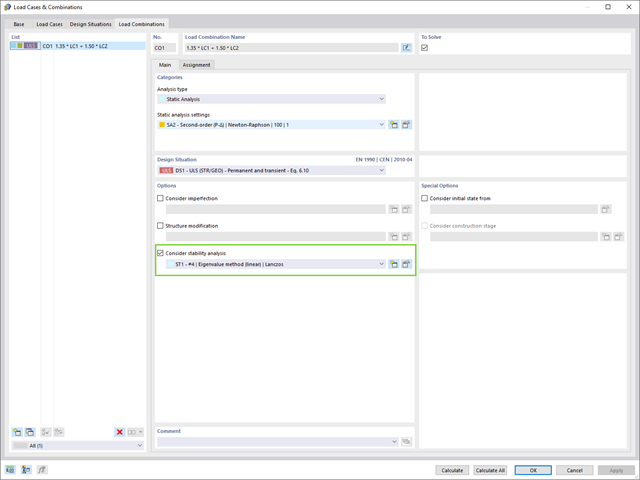
Jeżeli w programie istnieje przypadek obciążenia lub kombinacja obciążeń, obliczenia stateczności są aktywowane. Można zdefiniować inny przypadek obciążenia, na przykład w celu uwzględnienia naprężenia początkowego.
W tym celu należy określić, czy ma zostać przeprowadzona analiza liniowa czy nieliniowa. W zależności od przypadku zastosowania, można wybrać bezpośrednią metodę obliczeniową, taką jak metoda Lanczosa lub metoda iteracji ICG. Pręty niezintegrowane z powierzchniami są zazwyczaj wyświetlane jako elementy prętowe z dwoma węzłami ES. W przypadku zastosowania takich elementów program nie może określić wyboczenia lokalnego pojedynczych prętów. Z tego względu'istnieje możliwość automatycznego dzielenia prętów.
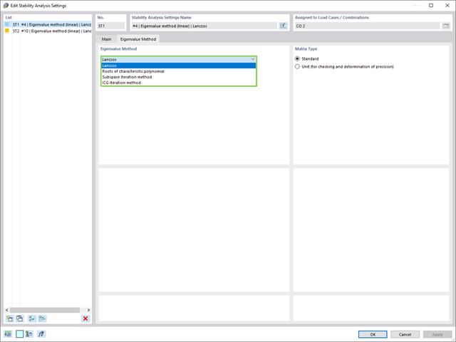
W przypadku analizy wartości własnych dostępnych jest kilka metod:
- Metody bezpośrednie
- Metody bezpośrednie (Lanczosa [RFEM], pierwiastki z wielomianu charakterystycznego [RFEM], metoda iteracji podprzestrzeni [RFEM/RSTAB], przesunięta iteracja odwrócona [RSTAB]) są odpowiednie dla małych i średnich modeli. Z szybkich metod rozwiązywania problemów należy korzystać tylko w przypadku, gdy komputer posiada dużą ilość pamięci RAM.
- Metoda iteracji ICG (niekompletny sprzężony gradient [RFEM])
- Z drugiej strony, ta metoda wymaga tylko niewielkiej ilości pamięci. Wartości własne są określane jedna po drugiej. Może być stosowany do obliczania dużych układów konstrukcyjnych o niewielkiej liczbie wartości własnych.
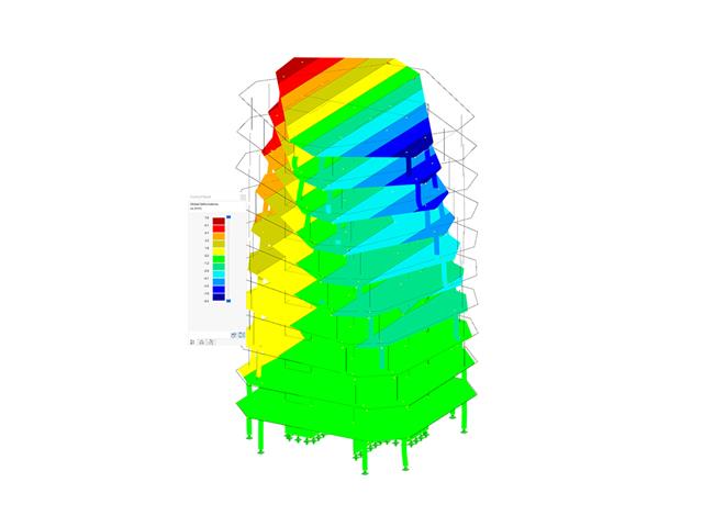
Rozszerzenie Stateczność konstrukcji umożliwia nieliniową analizę stateczności przy użyciu metody przyrostowej. Analiza ta dostarcza wyniki zbliżone do rzeczywistości również w przypadku konstrukcji nieliniowych. Współczynnik obciążenia krytycznego jest określany poprzez stopniowe zwiększanie obciążeń w podstawowym przypadku obciążenia, aż do osiągnięcia niestateczności. Przyrost obciążenia uwzględnia nieliniowości, takie jak ulegające uszkodzeniu pręty, podpory i fundamenty oraz nieliniowości materiałowe. Po zwiększeniu obciążenia można opcjonalnie przeprowadzić liniową analizę stateczności na ostatnim stabilnym stanie w celu określenia postaci stateczności.
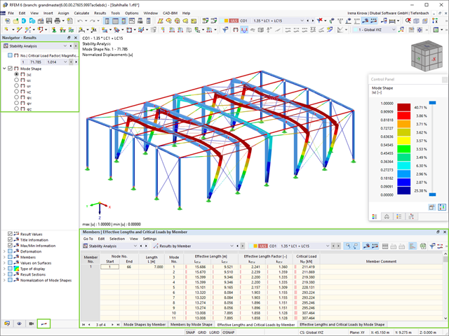
Jako pierwsze wyniki program przedstawia współczynniki obciążenia krytycznego. Następnie można przeprowadzić ocenę zagrożeń stateczności. W przypadku modeli prętowych w tabelach wyświetlane są wynikowe długości efektywne i obciążenia krytyczne prętów.
W następnym oknie wyników można sprawdzić znormalizowane wartości własne posortowane według węzła, pręta i powierzchni. Grafika wartości własnych umożliwia ocenę zachowania wyboczeniowego. Ułatwia to podjęcie środków zaradczych.
- 002073
- Ogólne informacje
- Analiza stateczności konstrukcji RFEM 6
- Analiza stateczności konstrukcji RSTAB 9
- Obliczanie modeli składających się z elementów prętowych, powłokowych i bryłowych
- Nieliniowa analiza stateczności
- Możliwość uwzględniania sił osiowych od wstępnego sprężenia
- Cztery dostępne solvery do rozwiązywania równań dla efektywnego obliczania różnych modeli konstrukcyjnych
- Opcjonalne uwzględnianie zmian w sztywności w programie RFEM/RSTAB
- Wyszukiwanie postaci wyboczeniowych o krytycznym mnożniku obciążenia większym niż zadany przez użytkownika (metoda "przesunięcia")
- Możliwość określania wektorów własnych dla modeli niestatecznych (w celu zidentyfikowania przyczyny niestateczności)
- Wizualizacja postaci niestateczności
- Podstawa określania imperfekcji
- Proste definiowanie etapów budowy konstrukcji w RFEM wraz z wizualizacją
- Dodawanie, usuwanie, modyfikowanie i reaktywacja elementów prętowych, powierzchniowych i bryłowych oraz ich właściwości (np. przeguby prętowe i liniowe, stopnie swobody dla podpór itp.)
- Ręczna oraz automatyczna kombinatoryka obciążeń na poszczególnych etapach budowy konstrukcji (np. w celu uwzględnienia obciążeń montażowych, tymczasowych urządzeń dźwigowych itp.)
- Uwzględnienie wpływów nieliniowych, takich jak uszkodzenie prętów rozciąganych lub nieliniowe zachowanie podpór
- Interakcja z innymi rozszerzeniami, takimi jak z. B. Nieliniowe zachowanie materiału, Stateczność konstrukcji, -rstab-9/additional-analyses/form-finding/form-finding itd.
- Wyświetlanie wyników w postaci numerycznej i graficznej dla poszczególnych etapów budowy
- Szczegółowy protokół wydruku wraz z dokumentacją wszystkich danych konstrukcyjnych i obciążeń dla każdego etapu budowy
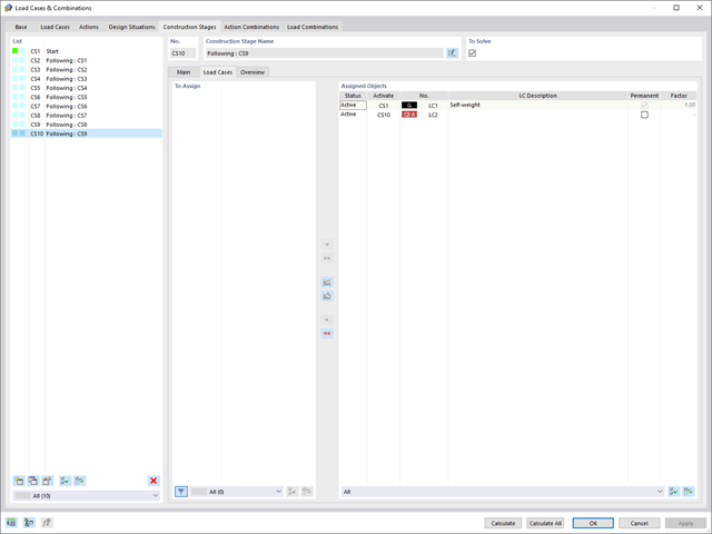
Czy udało Ci się utworzyć całą konstrukcję w programie RFEM? Dobrze, teraz można przypisać poszczególne elementy konstrukcyjne i przypadki obciążeń do odpowiednich etapów budowy. Na każdym etapie budowy można modyfikować na przykład definicje zwolnień prętów i podpór.
Pozwala to na modelowanie zmian konstrukcyjnych, na przykład podczas betonowania dźwigarów mostowych lub osiadania słupów. Przypadki obciążeń utworzone w programie RFEM należy następnie przydzielić do etapów budowy jako obciążenia stałe lub przejściowe.
Czy wiecie, że...? Kombinatoryka umożliwia nakładanie obciążeń stałych i przejściowych w kombinacjach obciążeń. W ten sposób można określić maksymalne siły wewnętrzne dla różnych pozycji dźwigu lub uwzględnić tymczasowe obciążenia montażowe dostępne tylko w jednym etapie budowy.
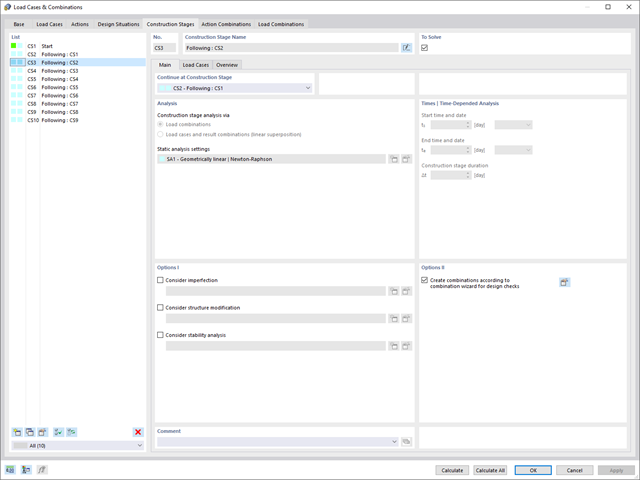
Jeżeli między idealnym układem a układem, który uległ deformacji z poprzedniego etapu budowy, pojawią się różnice w geometrii, są one porównywane w programie. Następujące po sobie kolejne etapy budowy obliczane są na bazie układu konstrukcyjnego z odkształceniami i obciążeniami wynikającymi z poprzednich etapu budowy. Obliczenia te są nieliniowe.
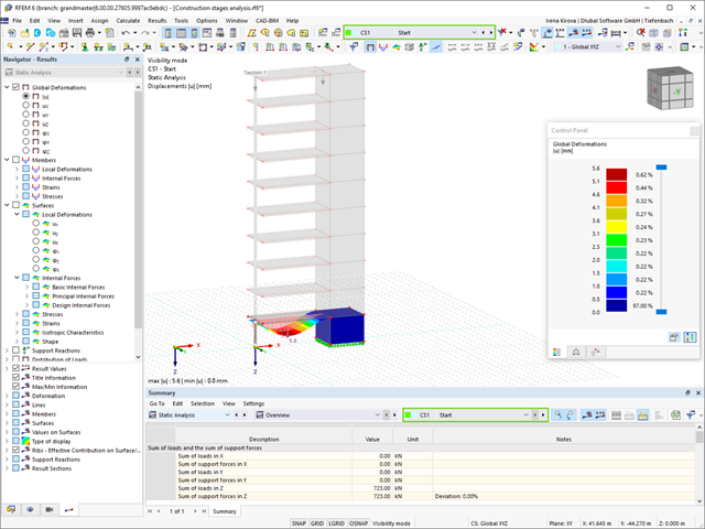
Czy obliczenia zakończyły się pomyślnie? Wyniki poszczególnych etapów budowy można teraz wyświetlać graficznie oraz w tabelach w programie RFEM. Ponadto program RFEM umożliwia uwzględnienie etapów budowy w kombinatoryce i uwzględnienie ich w dalszych obliczeniach.
_ENG.png?mw=640&hash=1053c9bef400e9f5361c9c3278f76a272fcc4ddf)
Czy aktywowałeś rozszerzenie Analiza historii czasowej (TDA)? Dobrze, teraz można dodawać dane czasowe do przypadków obciążeń. Po zdefiniowaniu początku i końca obciążenia, uwzględniany jest wpływ pełzania na końcu obciążenia. Program umożliwia modelowanie efektów pełzania w konstrukcjach szkieletowych i kratowych wykonanych z betonu zbrojonego.
W tym przypadku obliczenia są przeprowadzane nieliniowo zgodnie z modelem reologicznym (model Kelvina i Maxwella).
Czy obliczenia zakończyły się pomyślnie? Wyznaczone siły wewnętrzne można teraz wyświetlić w tabelach i grafice, a także uwzględnić w obliczeniach.

- Definiowanie naprężeń na przykładzie sprężysto-plastycznego modelu materiałowego
- Wymiarowanie murowych konstrukcji tarczowych na ściskanie i ścinanie na modelu budynku lub na pojedynczym modelu
- Automatyczne określanie sztywności przegubu ściana-płyta
- Obszerna baza danych materiałów o prawie wszystkich kombinacjach kamienia i zapraw dostępnych na rynku austriackim (asortyment jest stale poszerzany, również dla innych krajów)
- Automatyczne określanie wartości materiałów zgodnie z Eurokodem 6 (ÖN EN 1996‑X)
- Możliwość przeprowadzenia analizy pushover