49 Wyniki
Wyświetl wyniki:
Sortuj według:
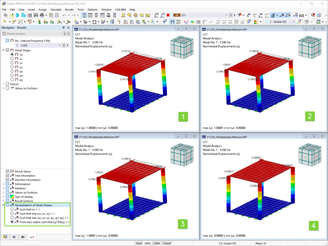
Jak już wiesz, po pomyślnym zakończeniu obliczeń wyniki przypadku obciążenia w Analizie modalnej są wyświetlane w programie. Die erste Eigenform ist für Sie also sofort grafisch oder animiert zu sehen. Dabei können Sie die Darstellung der Eigenformnormierung komfortabel anpassen. Erledigen Sie das am besten direkt im Ergebnisnavigator, wo Sie zur Visualisierung der Eigenformen eine von vier Optionen auswählen:
- Wert des Eigenformvektors uj auf 1 skalieren (berücksichtigt nur die Translationskomponenten)
- Auswahl der maximalen Translationskomponente des Eigenvektors und Einstellung auf 1
- Betrachtung der gesamten Eigenform (inklusive der Rotationskomponenten), Auswahl des Maximums und Einstellung auf 1
- Setzen der modalen Massen mi für jeden Eigenwert auf 1 kg
Ausführlichere Erläuterungen der Normierung der Eigenformen finden Sie hier: Instrukcja online .
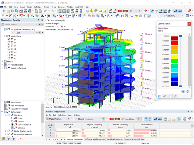
Czy obliczenia się zakończyły? Wyniki analizy modalnej są wówczas dostępne zarówno w formie graficznej, jak i tabelarycznej. Wyświetl tabele wyników dla przypadku obciążenia lub przypadków obciążeń analizy modalnej. Dzięki temu na pierwszy rzut oka można zobaczyć wartości własne, częstotliwości kątowe, częstotliwości i okresy drgań własnych konstrukcji. W przejrzysty sposób wyświetlane są również efektywne masy modalne, modalne współczynniki masy i współczynniki udziału.

- 002090
- Ogólne informacje
- Skręcanie skrępowane (7 stopni swobody) RFEM 6
- Skręcanie skrępowane (7 stopni swobody) RSTAB 9
Obliczenia skręcania skrępowanego można przeprowadzić dla całego układu. Uwzględniasz zatem dodatkową wartość 7 stopnia swobody w obliczeniach pręta. Sztywności połączonych elementów konstrukcyjnych są uwzględniane automatycznie. Oznacza to, że nie ma potrzeby' definiowania równoważnych sztywności sprężystych ani warunków podparcia dla układu odłączanego.
Następnie można wykorzystać siły wewnętrzne z obliczeń ze skręcaniem skrępowanym w rozszerzeniu do obliczeń. W zależności od materiału i wybranej normy należy uwzględnić bimoment wyboczeniowy i drugorzędny moment skręcający. Typowym zastosowaniem jest analiza stateczności według teorii drugiego rzędu z wykorzystaniem imperfekcji w konstrukcjach stalowych.
Czy wiecie, że...? Zastosowanie nie ogranicza się do przekrojów stalowych cienkościennych. Pozwala to na przykład na przeprowadzenie obliczeń idealnego momentu krytycznego dla belek o przekrojach z drewna litego.
- 002165
- Ogólne informacje
- Skręcanie skrępowane (7 stopni swobody) RFEM 6
- Skręcanie skrępowane (7 stopni swobody) RSTAB 9
W porównaniu z modułem dodatkowym RF-/STEEL Warping Torsion (RFEM 5/RSTAB 8) do rozszerzenia Skręcanie skrępowane (7 DOF) dla programu RFEM 6/RSTAB 9 dodano następujące nowe funkcje:
- Pełna integracja ze środowiskiem RFEM 6 i RSTAB 9
- Siódmy stopień swobody jest bezpośrednio uwzględniany w obliczeniach prętów w programie RFEM/RSTAB na całym układzie
- Nie ma już potrzeby definiowania warunków podparcia lub sztywności sprężystej do obliczeń w uproszczonym układzie zastępczym
- Możliwość łączenia z innymi rozszerzeniami, na przykład do obliczania obciążeń krytycznych dla wyboczenia skrętnego i zwichrzenia z analizą stateczności
- Brak ograniczeń dla stalowych przekrojów cienkościennych (możliwe jest również obliczenie momentu krytycznego, na przykład dla belek o masywnych przekrojach drewnianych)
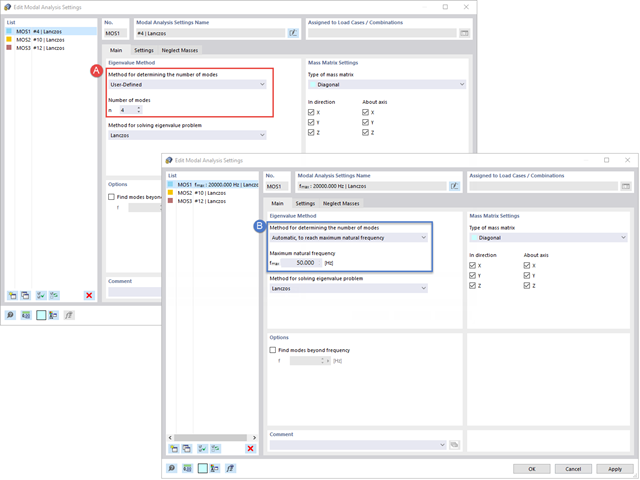
Twoim celem jest określenie liczby postaci drgań własnych? Program oferuje dwie metody. Z jednej strony, można ręcznie zdefiniować liczbę najmniejszych kształtów drgań, które mają zostać obliczone. W tym przypadku liczba dostępnych kształtów postaci zależy od stopni swobody (tzn. liczby punktów mas swobodnych pomnożonych przez liczbę kierunków, w których działają masy). Jest to jednak ograniczone do 9999. Z drugiej strony, maksymalną częstotliwość drgań własnych można ustawić w taki sposób, w jaki program określił kształty automatycznie, aż do osiągnięcia zadanej częstotliwości drgań własnych.
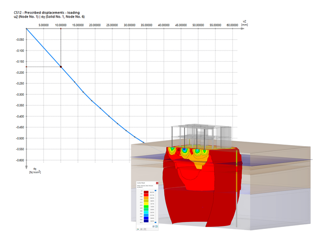
Czy jesteś gotowy na ocenę? Skorzystaj z wykresów obliczeniowych, które pokazują rozkład określonego wyniku podczas obliczeń.
Przypisanie osi pionowej i poziomej wykresu obliczeniowego można dowolnie definiować. Umożliwia to np. wyświetlenie przebiegu osiadania określonego węzła w zależności od obciążenia.
- 002089
- Ogólne informacje
- Skręcanie skrępowane (7 stopni swobody) RFEM 6
- Skręcanie skrępowane (7 stopni swobody) RSTAB 9
- Uwzględnienie 7 lokalnych kierunków deformacji (ux , uy, uz, φx, φy, φz, ω ) lub 8 sił wewnętrznych (N , Vu, Vv, Mt, pri, Mt, s, Mu, Mv, Mω ) przy obliczaniu elementów prętowych
- Możliwość stosowania w połączeniu z analizą statyczno-wytrzymałościową według teorii II rzędu, i analiza dużych deformacji (można również uwzględnić imperfekcje)
- W połączeniu z rozszerzeniem Analiza stateczności umożliwia definiowanie współczynników obciążenia krytycznego i kształtów drgań dla problemów stateczności, takich jak wyboczenie skrętne i zwichrzenie
- Uwzględnianie blach czołowych i usztywnień poprzecznych jako sprężystości skrępowanej podczas obliczania przekrojów dwuteowych z automatycznym określaniem i wyświetlaniem graficznym sztywności sprężystości deplanacyjnej
- Graficzne przedstawienie deplanacji przekroju prętów w stanie odkształcenia
- Pełna integracja z RFEM i RSTAB
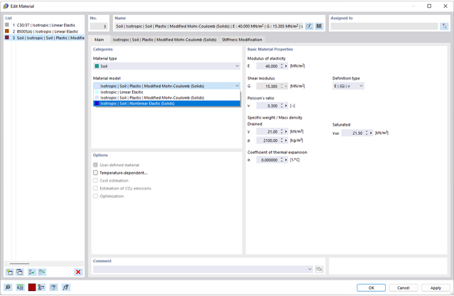
Czy chcesz modelować i analizować zachowanie bryły gruntowej? Aby to zapewnić, w programie RFEM zaimplementowano odpowiednie modele materiałowe.
Można użyć zmodyfikowanego modelu Mohra-Coulomba z liniowo-sprężystym modelem idealnie plastycznym lub nieliniowo sprężystym modelem z edometryczną relacją naprężenie-odkształcenie. Kryterium graniczne, które opisuje przejście od obszaru sprężystości do obszaru płynięcia plastycznego, jest zdefiniowane według Mohra-Coulomba.
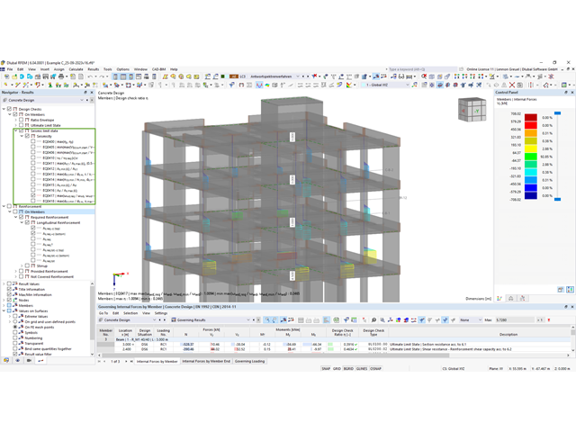
W rozszerzeniu Projektowanie konstrukcji betonowych można przeprowadzać obliczenia sejsmiczne dla prętów żelbetowych zgodnie z EC 8. Są to między innymi następujące funkcje:
- Konfiguracje obliczeń sejsmicznych
- Rozróżnianie klas ciągliwości DCL, DCM, DCH
- Możliwość przeniesienia współczynnika odpowiedzi z analizy dynamicznej
- Sprawdzenie wartości granicznej współczynnika odpowiedzi
- Weryfikacja nośności dla "Wytrzymały słup - słaba belka"
- Uszczegółowienie i reguły szczególne dla współczynnika ciągliwości krzywizny
- Uszczegółowienie i reguły szczególne dla ciągliwości lokalnej

W porównaniu z modułem dodatkowym RF-SOILIN (RFEM 5) do rozszerzenia Analiza geotechniczna dla programu RFEM 6 dodano następujące nowe funkcje:
- Tworzenie warstwowego gruntu jako modelu 3D z całości zdefiniowanych próbek gruntu
- Symulacja gruntu zgodnie z teorią Mohra-Coulomba
- Graficzne i tabelaryczne przedstawienie naprężeń i odkształceń na dowolnej głębokości gruntu
- Optymalne uwzględnienie interakcji gruntu i konstrukcji na podstawie modelu ogólnego
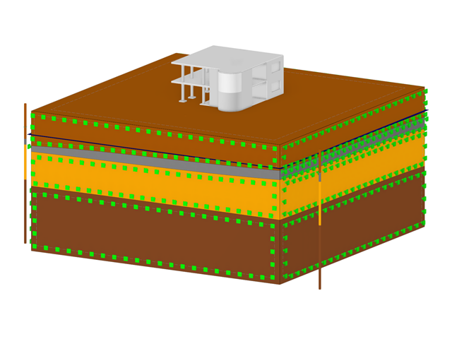
Bryły gruntu, które mają zostać przeanalizowane, są sumowane w masywach gruntu.
Próbki gruntu należy wykorzystać jako podstawę do zdefiniowania masywu gruntowego. W ten sposób program umożliwia generowanie masywu w sposób przyjazny dla użytkownika, w tym automatyczne określanie granic faz na podstawie danych z próbki, a także poziomu wód gruntowych i podpór powierzchni granicznej.
Masywy gruntowe umożliwiają określenie docelowego rozmiaru siatki ES niezależnie od ustawień globalnych dla reszty konstrukcji. Dzięki temu w całym modelu można uwzględnić różne wymagania dotyczące budynku i gruntu.
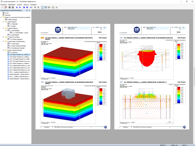
Twoje dane są zawsze dokumentowane w wielojęzycznym raporcie. W każdej chwili możesz dostosować treść i zapisać ją jako szablon. W raporcie można również za pomocą kilku kliknięć umieścić grafiki, teksty, wzory MathML i dokumenty PDF.
- 002401
- Ogólne informacje
- Skręcanie skrępowane (7 stopni swobody) RFEM 6
- Skręcanie skrępowane (7 stopni swobody) RSTAB 9
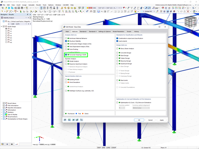
- Funkcję skręcania skrępowanego można aktywować lub dezaktywować w zakładce Rozszerzenia w Danych podstawowych modelu.
- Po aktywowaniu rozszerzenia interfejs użytkownika w programie RFEM zostaje rozszerzony o nowe wpisy w nawigatorze, tabelach i oknach dialogowych.
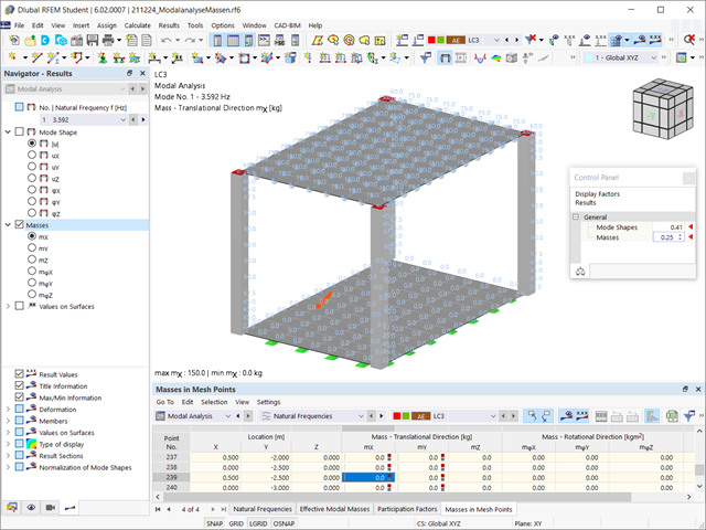
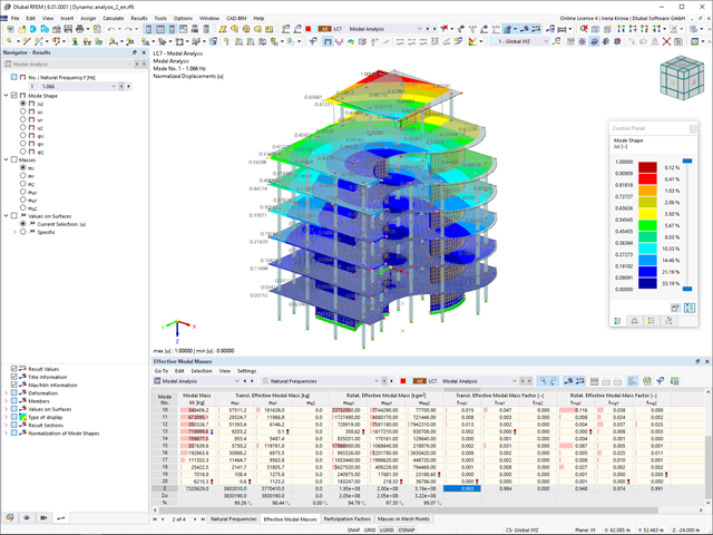
Czy odkryłeś już tabelaryczne i graficzne przedstawianie mas w punktach siatki? Po prawej, jest to również jeden z wyników analizy modalnej w programie RFEM 6. W ten sposób można sprawdzić importowane masy, które zależą od różnych ustawień analizy modalnej. Mogą być one wyświetlane w zakładce Masy w punktach siatki tabeli Wyniki. Tabela zawiera przegląd następujących wyników: Masa - kierunek przesuwny (mX, mY, mZ ), Masa - kierunek obrotowy (mφX, mφY, mφZ ) oraz suma mas. Czy nie byłoby lepiej, gdybyś jak najszybciej przeprowadził ocenę graficzną? Następnie można również wyświetlić graficznie masy w punktach siatki.
Wiesz już, że grunt i konstrukcję można modelować i analizować w całym modelu. Oznacza to, że wyraźnie uwzględniono interakcję gleba-konstrukcja. Dostosowanie jednego elementu konstrukcyjnego prowadzi do natychmiastowego prawidłowego uwzględnienia w analizie i wynikach dla całego układu gruntu i konstrukcji.
.png?mw=640&hash=55038d2a1591f62179796666cb9b2fede0274e19)
Graficzne i tabelaryczne wyświetlanie wyników dla deformacji, naprężeń i odkształceń pomaga określić bryłę gruntu. Aby to osiągnąć, skorzystaj ze specjalnych kryteriów filtrowania, które umożliwiają wybór określonych wyników.
Program na pewno cię nie zawiedzie. Jeśli chcesz graficznie ocenić wyniki w bryłach gruntu, dostępne są obiekty pomocnicze. Na przykład można zdefiniować płaszczyzny przycinania. Umożliwia to przeglądanie odpowiednich wyników na dowolnej płaszczyźnie bryły gruntu.
I nie tylko to. Wykorzystanie przekrojów wyników i brył przycinania ułatwia graficzną analizę brył gruntu.
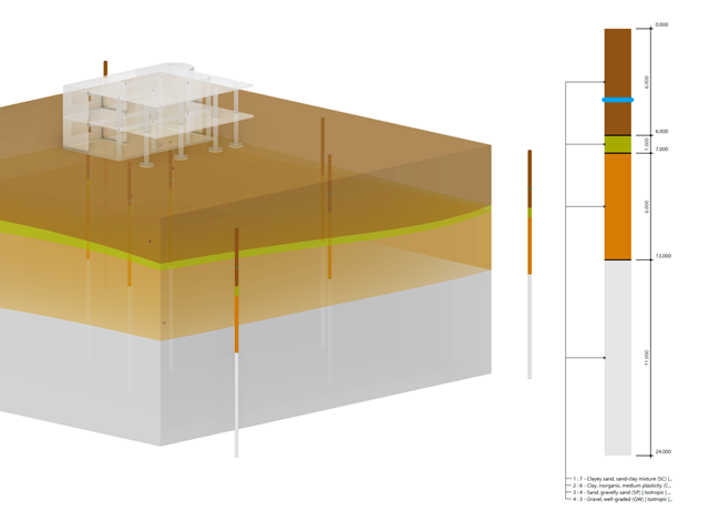
Czy wiecie, że...? Uwarstwienie gruntu, pobrane z raportów o podłożu gruntowym w miejscach wychodni, można wprowadzić bezpośrednio do programu w postaci próbek gruntu. Przypisz badane materiały gruntowe wraz z ich właściwościami do warstw.
Za pomocą danych tabelarycznych i okna dialogowego edycji można zdefiniować próbkę. Można również określić poziom wód gruntowych w próbkach gruntu.

- 002232
- Ogólne informacje
- Optymalizacja i koszty | Szacowanie emisji CO2 RFEM 6
- Optymalizacja i koszty | Szacowanie emisji CO2 RSTAB 9
Możesz być pewien, że koszty są ważnym czynnikiem w planowaniu konstrukcyjnym każdego projektu. Należy również przestrzegać przepisów dotyczących szacowania emisji. Dwuczęściowe rozszerzenie Optymalizacja i koszty/Szacowanie emisji CO2 ułatwia odnalezienie się w gąszczu norm i opcji. Wykorzystuje technologię sztucznej inteligencji (AI) optymalizacji rojem cząstek (PSO) w celu znalezienia odpowiednich parametrów dla sparametryzowanych modeli i bloków, które zagwarantują zgodność ze zwykłymi kryteriami optymalizacji. Ponadto, rozszerzenie oszacowuje koszty modelu lub emisję CO2 poprzez określenie kosztów jednostkowych lub emisji jednostkowej dla materiałów zdefiniowanych w modelu konstrukcyjnym. Dzięki temu rozszerzeniu jesteś po bezpiecznej stronie.
Wprowadzanie warstw gruntu dla potrzeb zadawania próbek gruntu odbywa się w przejrzystym oknie dialogowym. Odpowiadająca temu prezentacja graficzna zapewnia przejrzystość i ułatwia kontrolę wprowadzanych danych.
Rozszerzalna baza danych ułatwia wybór właściwości materiałowych dla gruntu. Dla realistycznego odwzorowania zachowania się materiału gruntowego można użyć modelu Mohra-Coulomba oraz model gruntu ze wzmocnieniem.
Można zdefiniować dowolną liczbę próbek i warstw gruntu. Grunt jest odwzorowany na podstawie wszystkich wprowadzonych próbek za pomocą brył 3D. Przypisanie do konstrukcji odbywa się za pomocą współrzędnych.
Zachowanie bryły gruntu jest obliczane za pomocą nieliniowej metody iteracyjnej. Obliczone naprężenia i osiadania są wyświetlane graficznie oraz w tabelach.
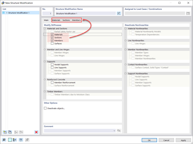
Czy wiecie, że...? W przypadkach obciążeń typu Analiza modalna można z łatwością wprowadzać zmiany konstrukcyjne. Pozwala to na przykład na indywidualne dostosowanie sztywności materiałów, przekrojów, prętów, powierzchni, przegubów i podpór. W przypadku niektórych rozszerzeń można również modyfikować sztywności. Po wybraniu obiektów ich właściwości sztywności są dostosowywane do typu obiektu. W ten sposób można je zdefiniować w osobnych zakładkach.
Czy chcesz przeanalizować uszkodzenie obiektu (na przykład słupa) w analizie modalnej? Jest to również możliwe bez żadnych problemów. Wystarczy przejść do okna Modyfikacja konstrukcji i dezaktywować odpowiednie obiekty.
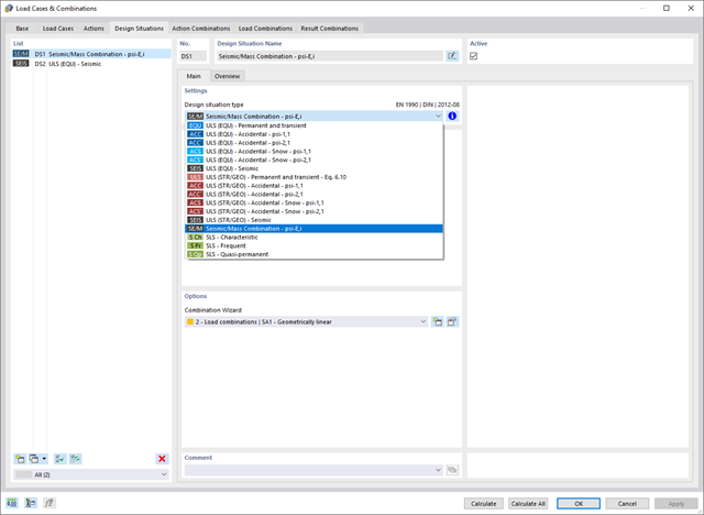
W porównaniu z modułem dodatkowym RF-/DYNAM Pro-Natural Vibrations (RFEM 5/RSTAB 8) do rozszerzenia Analiza modalna dla programu RFEM 6/RSTAB 9 dodano następujące nowe funkcje:
- Predefiniowane współczynniki kombinacji dla różnych norm (EC 8, ASCE itp.)
- Opcjonalne pominięcie mas (na przykład masy fundamentów)
- Metody określania liczby postaci drgań własnych (liczba zdefiniowana przez użytkownika, liczba określana automatycznie - w celu osiągnięcia zadanych efektywnych współczynników masy modalnej, liczba określana automatycznie - w celu osiągnięcia maksymalnej częstotliwości drgań własnych)
- Wyniki w postaci mas modalnych, efektywnych mas modalnych, współczynników masy modalnej i współczynników udziału masy
- Tabelaryczne i graficzne przedstawienie mas w punktach siatki MES
- Różne opcje skalowania postaci drgań własnych w nawigatorze wyników
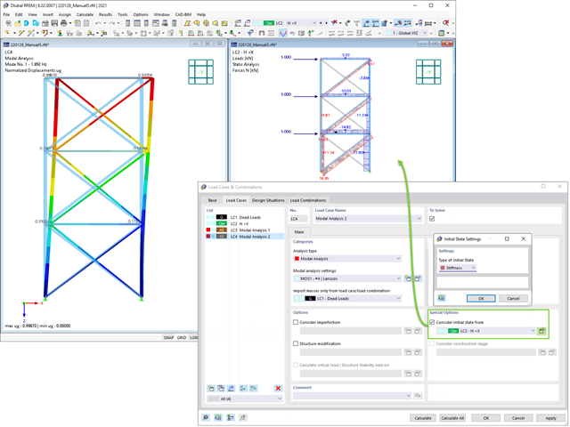
Podczas definiowania danych wejściowych dla przypadku obciążenia analizy modalnej można uwzględnić przypadek obciążenia, którego sztywności reprezentują początkową pozycję analizy modalnej. Jak to zrobić? Jak pokazano na rysunku, należy wybrać opcję "Uwzględnij stan początkowy z". Teraz otwórz okno dialogowe "Ustawienia stanu początkowego" i zdefiniuj typ Sztywność jako stan początkowy. W tym przypadku obciążenia, który jest stanem początkowym branym pod uwagę, można uwzględnić sztywność układu konstrukcyjnego, gdy pręty rozciągane ulegają uszkodzeniu. Celem tego wszystkiego: Sztywność z tego przypadku obciążenia jest uwzględniana w analizie modalnej. W ten sposób uzyskuje się wyraźnie elastyczny system.
Zaraz po zakończeniu obliczeń wyświetlane są wartości własne, częstotliwości drgań własnych i okresy. Okna z tymi wynikami zintegrowane są z programem głównym RFEM/RSTAB. W tabelach można znaleźć wszystkie kształty drgań konstrukcji, a także można je wyświetlić graficznie i animować.
Wszystkie tabele wyników i grafiki stanowią część raportu programu RFEM/RSTAB. Zapewnia to przejrzystą dokumentację obliczeń. Tabele można również eksportować do programu MS Excel.
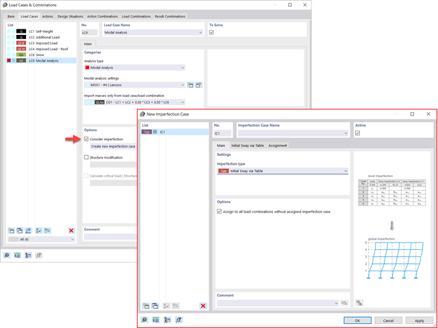
Widać to już na obrazku: Imperfekcje można również uwzględnić podczas definiowania przypadku obciążenia w analizie modalnej. Typy imperfekcji, które mogą być stosowane w analizie modalnej, to obciążenia hipotetyczne z przypadku obciążenia, początkowe przemieszczenie w tabeli, odkształcenie statyczne, postać wyboczeniowa, postać dynamiczna oraz grupa przypadków imperfekcji.
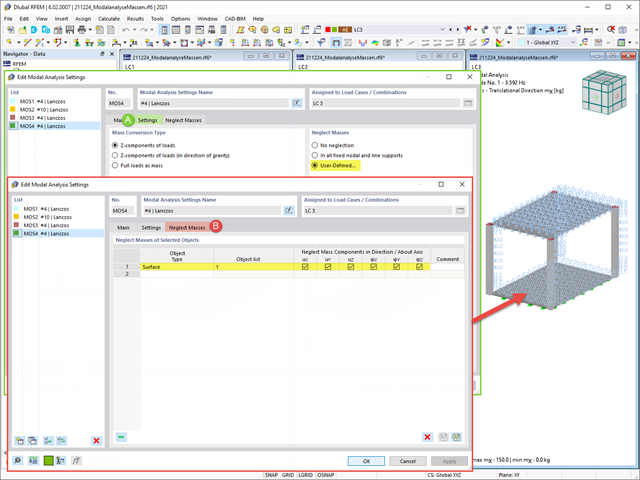
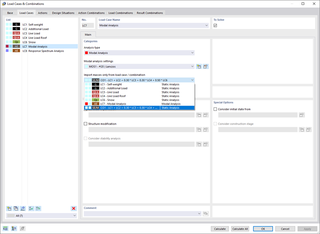
Często zachodzi potrzeba pominięcia mas. Dzieje się tak zwłaszcza w przypadku, gdy wyniki analizy modalnej mają być wykorzystane do analizy sejsmicznej. W tym celu wymagane jest 90% efektywnej masy modalnej w każdym kierunku. Pozwala to na pominięcie masy we wszystkich utwierdzonych podporach węzłowych i liniowych. Program automatycznie dezaktywuje powiązane masy.
Obiekty, których masy mają zostać pominięte w analizie modalnej, można również wybrać ręcznie. Dla lepszego widoku pokazaliśmy to ostatnie na rysunku. W wyniku wyboru przez użytkownika obiektów masowych wraz z skojarzonymi z nimi składowymi masowymi można pominąć masy.
_ENG.png?mw=640&hash=1053c9bef400e9f5361c9c3278f76a272fcc4ddf)
Czy aktywowałeś rozszerzenie Analiza historii czasowej (TDA)? Dobrze, teraz można dodawać dane czasowe do przypadków obciążeń. Po zdefiniowaniu początku i końca obciążenia, uwzględniany jest wpływ pełzania na końcu obciążenia. Program umożliwia modelowanie efektów pełzania w konstrukcjach szkieletowych i kratowych wykonanych z betonu zbrojonego.
W tym przypadku obliczenia są przeprowadzane nieliniowo zgodnie z modelem reologicznym (model Kelvina i Maxwella).
Czy obliczenia zakończyły się pomyślnie? Wyznaczone siły wewnętrzne można teraz wyświetlić w tabelach i grafice, a także uwzględnić w obliczeniach.
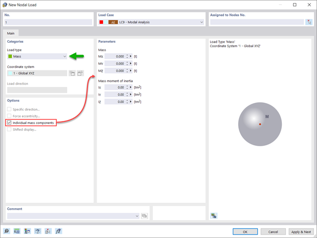
Czy oprócz obciążeń statycznych chcesz uwzględnić również inne obciążenia jako masy? Program umożliwia to dla obciążeń węzłowych, prętowych, liniowych i powierzchniowych. W tym celu podczas definiowania obciążenia należy wybrać typ Obciążenie masą. Dla takich obciążeń należy zdefiniować masę lub składowe masy w kierunkach X, Y i Z. W przypadku mas węzłowych można dodatkowo zdefiniować momenty bezwładności X, Y i Z w celu modelowania bardziej złożonych punktów mas.
W ustawieniach analizy modalnej należy wprowadzić wszystkie dane, które są niezbędne do określenia częstotliwości drgań własnych. Są to na przykład kształty mas i solwery wartości własnych.
Rozszerzenie Analiza modalna określa najniższe wartości częstości drgań własnych konstrukcji. Liczbę wartości własnych można dostosować lub określić automatycznie. Należy zatem osiągnąć efektywne współczynniki masy modalnej lub maksymalne częstotliwości drgań własnych. Masy są importowane bezpośrednio z przypadków obciążeń i kombinacji obciążeń. W takim przypadku istnieje możliwość uwzględnienia masy całkowitej, składowych obciążenia w globalnym kierunku Z lub tylko składowej obciążenia w kierunku siły ciężkości.
Dodatkowe masy w węzłach, liniach, prętach lub powierzchniach można zdefiniować ręcznie. Ponadto można wpływać na macierz sztywności poprzez import sił osiowych lub modyfikacji sztywności z przypadku obciążenia lub kombinacji obciążeń.

Dzięki rozszerzeniu Analiza historii czasowej (TDA) można uwzględnić zmienne w czasie zachowanie materiału w przypadku prętów i powierzchni. Długotrwałe efekty, takie jak pełzanie, skurcz i starzenie, mogą wpływać na rozkład sił wewnętrznych, w zależności od konstrukcji. Darauf bereiten Sie sich mit diesem Add-On optimal vor.
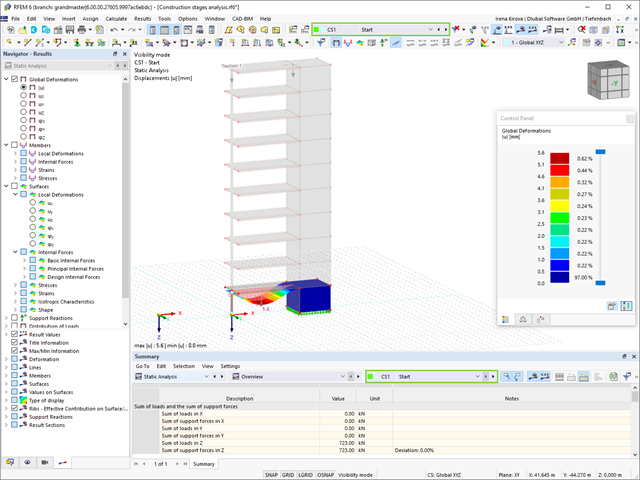
Czy obliczenia zakończyły się pomyślnie? Wyniki poszczególnych etapów budowy można teraz wyświetlać graficznie oraz w tabelach w programie RFEM. Ponadto program RFEM umożliwia uwzględnienie etapów budowy w kombinatoryce i uwzględnienie ich w dalszych obliczeniach.