36 Wyniki
Wyświetl wyniki:
Sortuj według:

W rozszerzeniu Analiza geotechniczna dostępny jest wysokiej jakości model materiałowy "Zmodyfikowany model gruntu twardniejącego". Ten model materiałowy jest odpowiedni dla różnych gruntów i jest w stanie odpowiednio odwzorować następujące właściwości rzeczywistego gruntu.
- Zależność naprężenia od sztywności gruntu
- Zależność ścieżki obciążenia od sztywności gruntu
- Odkształcenia plastyczne jeszcze przed osiągnięciem warunku granicznego
- Wzrost wytrzymałości na ścinanie wraz ze wzrostem zagęszczenia siatki
- Wzrost granicy plastyczności wraz ze wzrostem naprężenia, aż do osiągnięcia granicznego warunku plastyczności
- Kryterium uszkodzenia według Mohra-Coulomba
Więcej informacji na temat tego modelu materiałowego oraz definicji danych wejściowych w programie RFEM można znaleźć w odpowiednim rozdziale instrukcji online rozszerzenia Analiza geotechniczna.

- 002842
- Ogólne informacje
- Analiza naprężeniowo-odkształceniowa RFEM 6
- Analiza naprężeniowo-odkształceniowa RSTAB 9
W rozszerzeniu Analiza naprężeniowo-odkształceniowa można użyć opcji, aby określić zależne od znaku naprężenia graniczne za pomocą składowej naprężenia.

- 002829
- Ogólne informacje
- Analiza naprężeniowo-odkształceniowa RFEM 6
- Analiza naprężeniowo-odkształceniowa RSTAB 9
W rozszerzeniu Analiza naprężeniowo-odkształceniowa można zdefiniować cykl naprężeń granicznych zależny od elementu i uwzględnić go w obliczeniach.
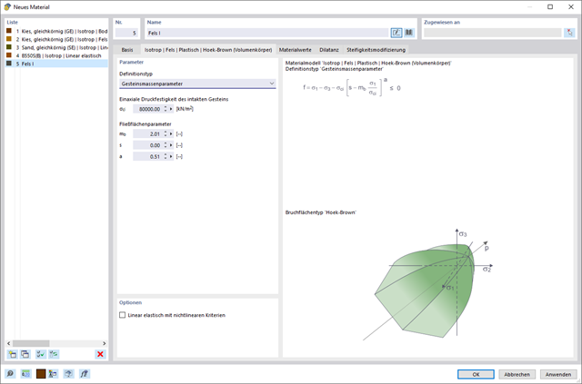
W rozszerzeniu Analiza geotechniczna dostępny jest model Hoek'a-Brown'a. Model wykazuje zachowanie materiału liniowo-sprężystego idealnie plastycznego. Jego nieliniowe kryterium wytrzymałości jest najczęściej stosowanym kryterium zniszczenia skał.
Parametry materiału można wprowadzić bezpośrednio za pomocą
- parametrów skały lub alternatywnie poprzez
- klasyfikację GSI.
opisane.
Weiterführende Informationen zu diesem Materialmodell und der Definition der Eingabe in RFEM finden Sie im entsprechenden Kapitel im Online-Handbuch für das Add-On Geotechnische Analyse: Model Hoeka-Browna .
.png?mw=640&hash=403c565ab80c4dd45c2d1356634fb74a90428b70)
W bibliotece konstrukcji warstwowych dostępni są następujący producenci drewna klejonego krzyżowo:
- Binderholz (USA)
- KLH (USA, CAN)
- Kalesnikoff (USA, CAN)
- Nordic Structures (USA, CAN)
- Mercer Mass Timber
- SmartLam
- Sterling Structural
- Konstrukcje nośne wymienione w Lignatec wydanie 32 "Drewno klejone krzyżowo z produkcji szwajcarskiej"
Wczytanie konstrukcji z biblioteki konstrukcji warstw powoduje automatyczne przejęcie wszystkich istotnych parametrów. Biblioteka jest stale aktualizowana.
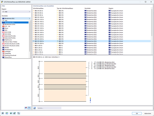
W programie RFEM zaimplementowano bibliotekę płyt z drewna klejonego krzyżowo, z której można importować konstrukcje warstwowe różnych producentów (np. Binderholz, KLH, Piveteaubois, Södra, Züblin Timber, Schilliger, Stora Enso). Oprócz grubości i materiałów warstw podane są również informacje o redukcji sztywności i łączeniu wąskich boków.
Przejdź do filmu.png?mw=640&hash=55038d2a1591f62179796666cb9b2fede0274e19)
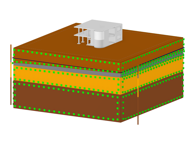
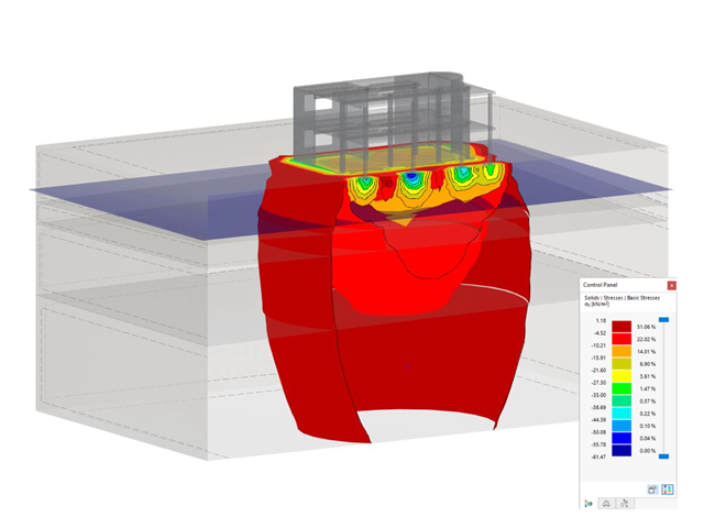
Graficzne i tabelaryczne wyświetlanie wyników dla deformacji, naprężeń i odkształceń pomaga określić bryłę gruntu. Aby to osiągnąć, skorzystaj ze specjalnych kryteriów filtrowania, które umożliwiają wybór określonych wyników.
Program na pewno cię nie zawiedzie. Jeśli chcesz graficznie ocenić wyniki w bryłach gruntu, dostępne są obiekty pomocnicze. Na przykład można zdefiniować płaszczyzny przycinania. Umożliwia to przeglądanie odpowiednich wyników na dowolnej płaszczyźnie bryły gruntu.
I nie tylko to. Wykorzystanie przekrojów wyników i brył przycinania ułatwia graficzną analizę brył gruntu.
Wiesz już, że grunt i konstrukcję można modelować i analizować w całym modelu. Oznacza to, że wyraźnie uwzględniono interakcję gleba-konstrukcja. Dostosowanie jednego elementu konstrukcyjnego prowadzi do natychmiastowego prawidłowego uwzględnienia w analizie i wynikach dla całego układu gruntu i konstrukcji.
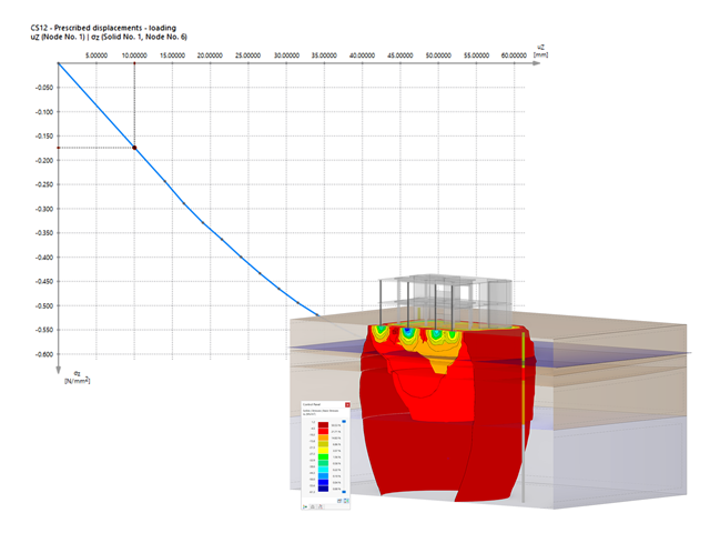
Czy jesteś gotowy na ocenę? Skorzystaj z wykresów obliczeniowych, które pokazują rozkład określonego wyniku podczas obliczeń.
Przypisanie osi pionowej i poziomej wykresu obliczeniowego można dowolnie definiować. Umożliwia to np. wyświetlenie przebiegu osiadania określonego węzła w zależności od obciążenia.
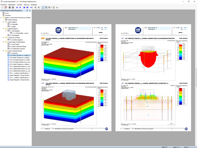
Twoje dane są zawsze dokumentowane w wielojęzycznym raporcie. W każdej chwili możesz dostosować treść i zapisać ją jako szablon. W raporcie można również za pomocą kilku kliknięć umieścić grafiki, teksty, wzory MathML i dokumenty PDF.
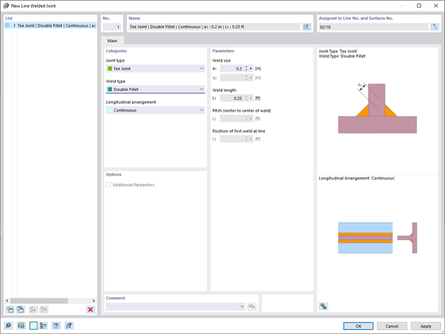
W programie RFEM 6 możliwe jest definiowanie spoin liniowych między powierzchniami i obliczanie naprężeń w spoinie za pomocą rozszerzenia Analiza naprężeniowo-odkształceniowa.
Dostępne są następujące typy połączeń:
- połączenie stykowe
- Złącze narożne
- Złącze zakładkowe
- Złącze teowe
W zależności od typu połączenia dostępne są następujące typy spoin:
- Pojedynczy kwadrat
- Podwójny
- Podwójny ukos
- Spoina typu V
- Spoina typu 2 V
- Spoina typu U
- Spoina typu 2 U
- Spoina typu J
- Spoina typu 2 J
Wprowadzenie i modelowanie bryły gruntowej bezpośrednio w programie RFEM. Modele materiałów gruntowych można łączyć ze wszystkimi popularnymi rozszerzeniami dla programu RFEM.
Umożliwia to łatwą analizę całych modeli z pełną prezentacją interakcji grunt-konstrukcja.
Wszystkie parametry wymagane do obliczeń są określane automatycznie na podstawie wprowadzonych danych materiałowych. Następnie program generuje krzywe naprężenie-odkształcenie dla każdego elementu ES.
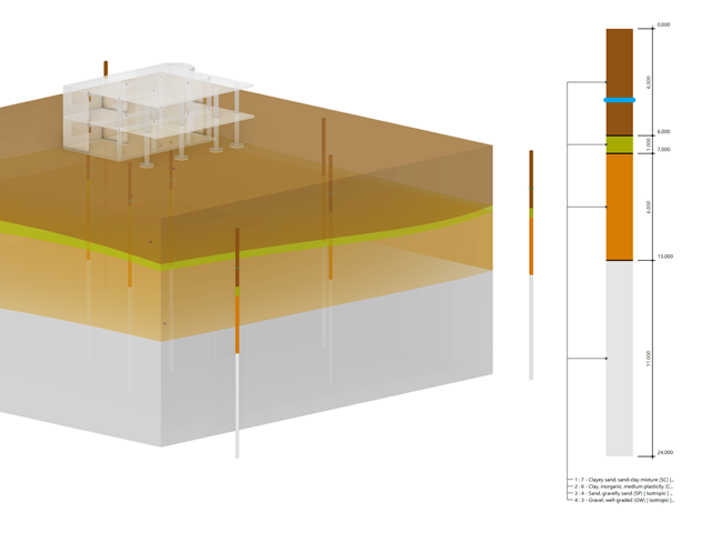
Czy wiecie, że...? Uwarstwienie gruntu, pobrane z raportów o podłożu gruntowym w miejscach wychodni, można wprowadzić bezpośrednio do programu w postaci próbek gruntu. Przypisz badane materiały gruntowe wraz z ich właściwościami do warstw.
Za pomocą danych tabelarycznych i okna dialogowego edycji można zdefiniować próbkę. Można również określić poziom wód gruntowych w próbkach gruntu.
Bryły gruntu, które mają zostać przeanalizowane, są sumowane w masywach gruntu.
Próbki gruntu należy wykorzystać jako podstawę do zdefiniowania masywu gruntowego. W ten sposób program umożliwia generowanie masywu w sposób przyjazny dla użytkownika, w tym automatyczne określanie granic faz na podstawie danych z próbki, a także poziomu wód gruntowych i podpór powierzchni granicznej.
Masywy gruntowe umożliwiają określenie docelowego rozmiaru siatki ES niezależnie od ustawień globalnych dla reszty konstrukcji. Dzięki temu w całym modelu można uwzględnić różne wymagania dotyczące budynku i gruntu.
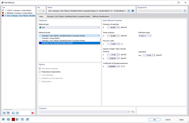
Czy chcesz modelować i analizować zachowanie bryły gruntowej? Aby to zapewnić, w programie RFEM zaimplementowano odpowiednie modele materiałowe.
Można użyć zmodyfikowanego modelu Mohra-Coulomba z liniowo-sprężystym modelem idealnie plastycznym lub nieliniowo sprężystym modelem z edometryczną relacją naprężenie-odkształcenie. Kryterium graniczne, które opisuje przejście od obszaru sprężystości do obszaru płynięcia plastycznego, jest zdefiniowane według Mohra-Coulomba.
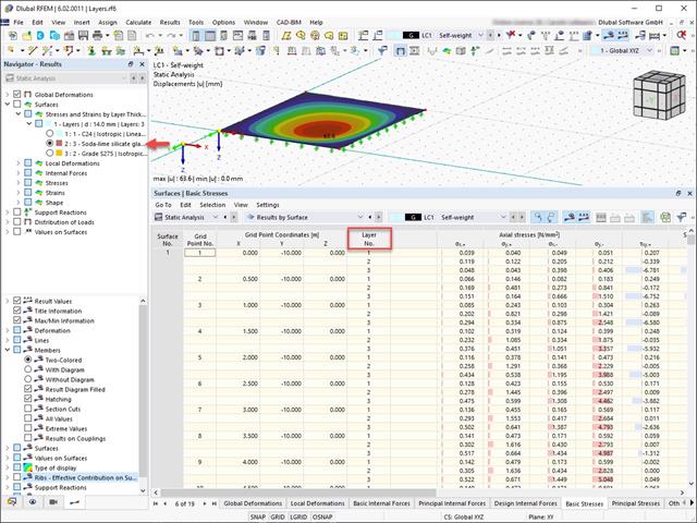
Wyniki naprężeń i odkształceń według powierzchni można wyświetlić w tabeli wyników powierzchni zgodnie z grubością warstwy.

- 002232
- Ogólne informacje
- Optymalizacja i koszty | Szacowanie emisji CO2 RFEM 6
- Optymalizacja i koszty | Szacowanie emisji CO2 RSTAB 9
Możesz być pewien, że koszty są ważnym czynnikiem w planowaniu konstrukcyjnym każdego projektu. Należy również przestrzegać przepisów dotyczących szacowania emisji. Dwuczęściowe rozszerzenie Optymalizacja i koszty/Szacowanie emisji CO2 ułatwia odnalezienie się w gąszczu norm i opcji. Wykorzystuje technologię sztucznej inteligencji (AI) optymalizacji rojem cząstek (PSO) w celu znalezienia odpowiednich parametrów dla sparametryzowanych modeli i bloków, które zagwarantują zgodność ze zwykłymi kryteriami optymalizacji. Ponadto, rozszerzenie oszacowuje koszty modelu lub emisję CO2 poprzez określenie kosztów jednostkowych lub emisji jednostkowej dla materiałów zdefiniowanych w modelu konstrukcyjnym. Dzięki temu rozszerzeniu jesteś po bezpiecznej stronie.

Dzięki rozszerzeniu Analiza historii czasowej (TDA) można uwzględnić zmienne w czasie zachowanie materiału w przypadku prętów i powierzchni. Długotrwałe efekty, takie jak pełzanie, skurcz i starzenie, mogą wpływać na rozkład sił wewnętrznych, w zależności od konstrukcji. Darauf bereiten Sie sich mit diesem Add-On optimal vor.
Dla każdego przypadku obciążenia można wyświetlić odkształcenia w czasie końcowym.
Wyniki te są również dokumentowane w protokole wydruku programów RFEM i RSTAB. Zawartość protokołu i jego zakres można wybrać specjalnie dla poszczególnych warunków projektowych.

- 002165
- Ogólne informacje
- Skręcanie skrępowane (7 stopni swobody) RFEM 6
- Skręcanie skrępowane (7 stopni swobody) RSTAB 9
W porównaniu z modułem dodatkowym RF-/STEEL Warping Torsion (RFEM 5/RSTAB 8) do rozszerzenia Skręcanie skrępowane (7 DOF) dla programu RFEM 6/RSTAB 9 dodano następujące nowe funkcje:
- Pełna integracja ze środowiskiem RFEM 6 i RSTAB 9
- Siódmy stopień swobody jest bezpośrednio uwzględniany w obliczeniach prętów w programie RFEM/RSTAB na całym układzie
- Nie ma już potrzeby definiowania warunków podparcia lub sztywności sprężystej do obliczeń w uproszczonym układzie zastępczym
- Możliwość łączenia z innymi rozszerzeniami, na przykład do obliczania obciążeń krytycznych dla wyboczenia skrętnego i zwichrzenia z analizą stateczności
- Brak ograniczeń dla stalowych przekrojów cienkościennych (możliwe jest również obliczenie momentu krytycznego, na przykład dla belek o masywnych przekrojach drewnianych)

W porównaniu z modułem dodatkowym RF-SOILIN (RFEM 5) do rozszerzenia Analiza geotechniczna dla programu RFEM 6 dodano następujące nowe funkcje:
- Tworzenie warstwowego gruntu jako modelu 3D z całości zdefiniowanych próbek gruntu
- Symulacja gruntu zgodnie z teorią Mohra-Coulomba
- Graficzne i tabelaryczne przedstawienie naprężeń i odkształceń na dowolnej głębokości gruntu
- Optymalne uwzględnienie interakcji gruntu i konstrukcji na podstawie modelu ogólnego
- 002169
- Ogólne informacje
- Analiza naprężeniowo-odkształceniowa RFEM 6
- Analiza naprężeniowo-odkształceniowa RSTAB 9
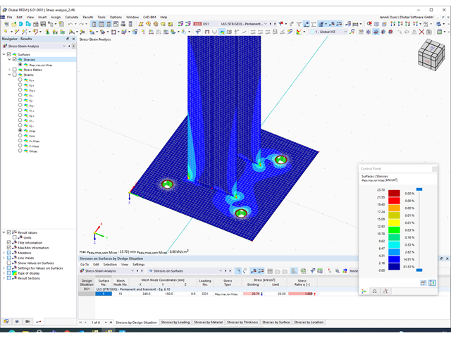
W porównaniu z modułem dodatkowym RF-/STEEL (RFEM 5/RSTAB 8) do rozszerzenia Analiza naprężeniowo-odkształceniowa dla programu RFEM 6/RSTAB 9 dodano następujące nowe funkcje:
- Możliwość analizy prętów, powierzchni, brył, spoin (połączenia spawane liniowo między dwiema i trzema powierzchniami z późniejszym obliczaniem naprężeń)
- Wyświetlanie naprężeń, stopni naprężeń, zakresów naprężeń i odkształceń
- Naprężenie graniczne w zależności od przydzielonego materiału lub danych wejściowych zdefiniowanych przez użytkownika
- Indywidualne określenie wyników do obliczeń poprzez dowolnie przydzielane typów ustawień
- Szczegóły dla wyników niemodalnych z wyświetlaniem przygotowanego wzoru i dodatkowym wyświetlaniem wyników na poziomie przekroju prętów
- Możliwość wygenerowania zastosowanych wzorów do kontroli obliczeń

- 002108
- Ogólne informacje
- Optymalizacja i koszty | Szacowanie emisji CO2 RFEM 6
- Optymalizacja i koszty | Szacowanie emisji CO2 RSTAB 9
- Technologia sztucznej inteligencji (AI): Optymalizacja roju cząstek (PSO)
- Optymalizacja konstrukcji ze względu na minimalny ciężar lub deformację
- Możliwość zastosowania dowolnej liczby parametrów optymalizacyjnych
- Określanie zakresów zmiennych
- Optymalizacja przekrojów i materiałów
- Typy definicji parametrów
- Optymalizacja | Rosnąco, czyli optymalizacja | Malejąca
- Zastosowanie parametrycznych modeli i bloków
- Parametryzacja bloków w języku JavaScript na podstawie kodu
- Optymalizacja z uwzględnieniem wyników obliczeń
- Tabelaryczne przedstawienie najlepszych mutacji modelu
- Wyświetlanie w czasie rzeczywistym mutacji modelu w procesie optymalizacji
- Kalkulacja kosztów modelu dzięki zadanym cenom jednostkowym
- Określanie potencjału tworzenia efektu cieplarnianego (GWP-global warming potential) na etapie tworzenia modelu poprzez szacowanie równoważnej emisji CO2
- Określanie jednostkowych wskaźników zależnych od masy, objętości i powierzchni (cena i emisja CO2)

- 002109
- Ogólne informacje
- Optymalizacja i koszty | Szacowanie emisji CO2 RFEM 6
- Optymalizacja i koszty | Szacowanie emisji CO2 RSTAB 9
Masz pytania dotyczące programu? Optymalizacja konstrukcji w programach RFEM i RSTAB jest uzupełnieniem parametrycznego wprowadzania danych. Jest to proces równoległy, niezależny od rzeczywistych obliczeń modelu wraz ze wszystkimi jego zwykłymi definicjami obliczeń i obliczeń. Rozszerzenie zakłada, że model lub blok jest zbudowany w kontekście parametrycznym i jest kontrolowany przez globalne parametry kontrolne typu "optymalizacja". Dlatego te parametry kontrolne mają dolną i górną granicę oraz wielkość kroku w celu ograniczenia zakresu optymalizacji. Aby znaleźć optymalne wartości parametrów kontrolnych, należy określić kryterium optymalizacji (na przykład minimalny ciężar) przy wyborze metody optymalizacji (na przykład optymalizacja roju cząstek).
Oszacowanie kosztów i emisji CO2 można znaleźć już w definicjach materiałów. Obie opcje można aktywować osobno w każdej definicji materiału. Oszacowanie oparte jest na koszcie jednostkowym lub jednostkowej wartości emisji dla prętów, powierzchni oraz brył. W tym przypadku można wybrać, czy jednostki mają zostać podane według masy, objętości czy powierzchni.

- 002110
- Ogólne informacje
- Optymalizacja i koszty | Szacowanie emisji CO2 RFEM 6
- Optymalizacja i koszty | Szacowanie emisji CO2 RSTAB 9
Istnieją dwie metody optymalizacji, dzięki którym można znaleźć optymalne wartości parametrów według kryterium ciężaru lub odkształcenia.
Najbardziej wydajną metodą o najkrótszym czasie obliczeń jest optymalizacja roju cząstek zbliżona do naturalnej (PSO). Czy słyszałeś lub czytałeś o tym? Ta technologia sztucznej inteligencji (AI) ma silną analogię do zachowania stad zwierząt szukających miejsca odpoczynku. W takich rojach można znaleźć wiele osób (por. rozwiązanie optymalizacyjne - na przykład waga), które lubią przebywać w grupie i podążać za ruchem grupy. Załóżmy, że każdy pręt roju musi zostać poddany spoczynkowi w optymalnym miejscu (por. najlepsze rozwiązanie - na przykład najniższa waga). Potrzeba ta wzrasta wraz ze zbliżaniem się do miejsca odpoczynku. Na zachowanie roju mają zatem wpływ również właściwości przestrzeni (por. wykres wyników).
Dlaczego wycieczka do biologii? Po prostu - proces PSO w RFEM lub RSTAB przebiega w podobny sposób. Proces obliczeń rozpoczyna się od wyniku optymalizacji poprzez losowe przypisanie parametrów, które mają zostać zoptymalizowane. Wielokrotnie określa nowe wyniki optymalizacji ze zróżnicowanymi wartościami parametrów, które opierają się na doświadczeniach z wcześniej przeprowadzonych mutacji modelu. Proces jest kontynuowany do momentu osiągnięcia określonej liczby możliwych mutacji modelu.
Jako alternatywa dla tej metody program oferuje również metodę przetwarzania wsadowego. Metoda ta ma na celu sprawdzenie wszystkich możliwych mutacji modelu poprzez losowe określanie wartości parametrów optymalizacji, aż do osiągnięcia określonej liczby możliwych mutacji modelu.
Po obliczeniu mutacji modelu obydwa warianty sprawdzają również odpowiednie aktywowane wyniki obliczeń rozszerzeń. Ponadto zapisuje on wariant z odpowiednim wynikiem optymalizacji i przypisaniem wartości parametrów optymalizacji, jeżeli wykorzystanie jest < 1.
Na podstawie odpowiednich sum poszczególnych materiałów można określić szacunkowe koszty całkowite i emisję. Na sumę materiałów składają się zależne od ciężaru, objętości i powierzchnie elementów prętowych, powierzchniowych i bryłowych.

- 002161
- Ogólne informacje
- Optymalizacja i koszty | Szacowanie emisji CO2 RFEM 6
- Optymalizacja i koszty | Szacowanie emisji CO2 RSTAB 9
Obie metody optymalizacji mają jedną wspólną cechę. Na końcu procesu wyświetlają listę wariacji modelu na podstawie przechowywanych danych. Można tu znaleźć szczegóły na temat wyniku decydującego dla optymalizacji i odpowiadające mu wartości parametrów. Lista jest zorganizowana w porządku malejącym. Zakładane najlepsze rozwiązanie znajduje się na górze. W takim przypadku wynik optymalizacji wraz z wyznaczoną wartością jest najbardziej zbliżony do kryterium optymalizacji. Wszystkie dodatkowe wyniki pokazują wykorzystanie < 1. Ponadto, po zakończeniu analizy, program dostosuje wartości na globalnej liście parametrów, aby odpowiadały tym dla optymalnego rozwiązania.
W oknach dialogowych materiałów znajdują się dodatkowe zakładki "Oszacowanie kosztów" i "Oszacowanie emisji CO2". Tutaj wyświetlane są indywidualne szacunkowe sumy przydzielonych prętów, powierzchni i objętości na jednostkę masy, objętości i powierzchni. Dodatkowo zakładki te podają całkowity koszt i emisję wszystkich przydzielonych do konstrukcji materiałów. Zapewnia to dobry przegląd projektu.
_ENG.png?mw=640&hash=1053c9bef400e9f5361c9c3278f76a272fcc4ddf)
Czy aktywowałeś rozszerzenie Analiza historii czasowej (TDA)? Dobrze, teraz można dodawać dane czasowe do przypadków obciążeń. Po zdefiniowaniu początku i końca obciążenia, uwzględniany jest wpływ pełzania na końcu obciążenia. Program umożliwia modelowanie efektów pełzania w konstrukcjach szkieletowych i kratowych wykonanych z betonu zbrojonego.
W tym przypadku obliczenia są przeprowadzane nieliniowo zgodnie z modelem reologicznym (model Kelvina i Maxwella).
Czy obliczenia zakończyły się pomyślnie? Wyznaczone siły wewnętrzne można teraz wyświetlić w tabelach i grafice, a także uwzględnić w obliczeniach.
- Realistyczne odwzorowanie interakcji między budynkiem a gruntem
- Realistyczne odwzorowanie oddziaływania poszczególnych fundamentów na siebie nawzajem
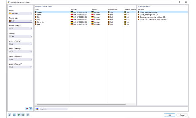
- Biblioteka parametrów gruntowych z możliwością rozszerzania
- Możliwość uwzględniania wielu próbek gruntu z różnych lokalizacji, także poza obrysem budynku
- Określanie osiadań oraz wykresów naprężeń w gruncie oraz ich prezentacja w formie graficznej i tabelarycznej
Wprowadzanie warstw gruntu dla potrzeb zadawania próbek gruntu odbywa się w przejrzystym oknie dialogowym. Odpowiadająca temu prezentacja graficzna zapewnia przejrzystość i ułatwia kontrolę wprowadzanych danych.
Rozszerzalna baza danych ułatwia wybór właściwości materiałowych dla gruntu. Dla realistycznego odwzorowania zachowania się materiału gruntowego można użyć modelu Mohra-Coulomba oraz model gruntu ze wzmocnieniem.
Można zdefiniować dowolną liczbę próbek i warstw gruntu. Grunt jest odwzorowany na podstawie wszystkich wprowadzonych próbek za pomocą brył 3D. Przypisanie do konstrukcji odbywa się za pomocą współrzędnych.
Zachowanie bryły gruntu jest obliczane za pomocą nieliniowej metody iteracyjnej. Obliczone naprężenia i osiadania są wyświetlane graficznie oraz w tabelach.
- 002089
- Ogólne informacje
- Skręcanie skrępowane (7 stopni swobody) RFEM 6
- Skręcanie skrępowane (7 stopni swobody) RSTAB 9
- Uwzględnienie 7 lokalnych kierunków deformacji (ux , uy, uz, φx, φy, φz, ω ) lub 8 sił wewnętrznych (N , Vu, Vv, Mt, pri, Mt, s, Mu, Mv, Mω ) przy obliczaniu elementów prętowych
- Możliwość stosowania w połączeniu z analizą statyczno-wytrzymałościową według teorii II rzędu, i analiza dużych deformacji (można również uwzględnić imperfekcje)
- W połączeniu z rozszerzeniem Analiza stateczności umożliwia definiowanie współczynników obciążenia krytycznego i kształtów drgań dla problemów stateczności, takich jak wyboczenie skrętne i zwichrzenie
- Uwzględnianie blach czołowych i usztywnień poprzecznych jako sprężystości skrępowanej podczas obliczania przekrojów dwuteowych z automatycznym określaniem i wyświetlaniem graficznym sztywności sprężystości deplanacyjnej
- Graficzne przedstawienie deplanacji przekroju prętów w stanie odkształcenia
- Pełna integracja z RFEM i RSTAB