113 Wyniki
Wyświetl wyniki:
Sortuj według:

- 002876
- Ogólne informacje
- Projektowanie konstrukcji betonowych RFEM 6
- Projektowanie konstrukcji betonowych RSTAB 9
Szczegółowe instrukcje dotyczące obliczeń są wyświetlane osobno, na podstawie obliczeń dotyczących konstrukcji.

W rozszerzeniu Połączenia stalowe można używać nie tylko zwykłych typów prętów 'Belka', 'Kratownica' itd., ale także typu pręta 'Belka wynikowa' oraz przekroje z elementów powierzchniowych. Należy wybrać odpowiedni przekrój dla belki wynikowej, a następnie zdefiniować otwory prętowe w modelu powierzchniowym za pomocą edytora prętów.

W rozszerzeniu Połączenie stalowe można rozmieszczać obiekty w odniesieniu do innych obiektów.

W rozszerzeniu Analiza geotechniczna dostępny jest wysokiej jakości model materiałowy "Zmodyfikowany model gruntu twardniejącego". Ten model materiałowy jest odpowiedni dla różnych gruntów i jest w stanie odpowiednio odwzorować następujące właściwości rzeczywistego gruntu.
- Zależność naprężenia od sztywności gruntu
- Zależność ścieżki obciążenia od sztywności gruntu
- Odkształcenia plastyczne jeszcze przed osiągnięciem warunku granicznego
- Wzrost wytrzymałości na ścinanie wraz ze wzrostem zagęszczenia siatki
- Wzrost granicy plastyczności wraz ze wzrostem naprężenia, aż do osiągnięcia granicznego warunku plastyczności
- Kryterium uszkodzenia według Mohra-Coulomba
Więcej informacji na temat tego modelu materiałowego oraz definicji danych wejściowych w programie RFEM można znaleźć w odpowiednim rozdziale instrukcji online rozszerzenia Analiza geotechniczna.

Komponent 'Kontakt powierzchniowy' w rozszerzeniu Połączenia stalowe umożliwia uwzględnienie kontaktu ciśnieniowego między dwiema równoległymi płytami/płytami prętowymi. W takim przypadku można opcjonalnie uwzględnić tarcie między powierzchniami

Komponent "Stub" jest dostępny w rozszerzeniu Połączenia stalowe. Umożliwia ona wydłużenie pręta za pomocą połączenia płatwi z innym prętem (krótkiem) i połączenie go z komponentem odniesienia.

W rozszerzeniu Połączenia stalowe można teraz układać płyty w różne kształty geometryczne. Oprócz „Prostokąta” i „Okręgu” dostępny jest nowy kształt „Wielokąt”. Forma wielokąta jest określana przez zdefiniowaną współrzędną punktu.

- 002161
- Ogólne informacje
- Optymalizacja i koszty | Szacowanie emisji CO2 RFEM 6
- Optymalizacja i koszty | Szacowanie emisji CO2 RSTAB 9
Obie metody optymalizacji mają jedną wspólną cechę. Na końcu procesu wyświetlają listę wariacji modelu na podstawie przechowywanych danych. Można tu znaleźć szczegóły na temat wyniku decydującego dla optymalizacji i odpowiadające mu wartości parametrów. Lista jest zorganizowana w porządku malejącym. Zakładane najlepsze rozwiązanie znajduje się na górze. W takim przypadku wynik optymalizacji wraz z wyznaczoną wartością jest najbardziej zbliżony do kryterium optymalizacji. Wszystkie dodatkowe wyniki pokazują wykorzystanie < 1. Ponadto, po zakończeniu analizy, program dostosuje wartości na globalnej liście parametrów, aby odpowiadały tym dla optymalnego rozwiązania.
W oknach dialogowych materiałów znajdują się dodatkowe zakładki "Oszacowanie kosztów" i "Oszacowanie emisji CO2". Tutaj wyświetlane są indywidualne szacunkowe sumy przydzielonych prętów, powierzchni i objętości na jednostkę masy, objętości i powierzchni. Dodatkowo zakładki te podają całkowity koszt i emisję wszystkich przydzielonych do konstrukcji materiałów. Zapewnia to dobry przegląd projektu.

W konfiguracji granicznej dla wymiarowania połączenia stalowego istnieje możliwość modyfikacji granicznego odkształcenia plastycznego dla spoin.
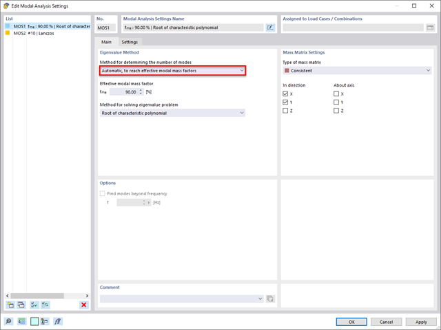
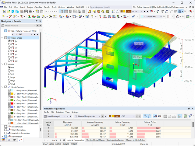
Rozszerzenie Analiza modalna umożliwia automatyczne zwiększanie poszukiwanych wartości własnych do momentu osiągnięcia zdefiniowanego współczynnika efektywnej masy modalnej. Uwzględniane są wszystkie kierunki translacyjne, które zostały aktywowane jako masy do analizy modalnej.
W ten sposób można łatwo obliczyć wymagane 90% efektywnej masy modalnej dla metody spektrum odpowiedzi.

W rozszerzeniu Projektowanie konstrukcji betonowych dla programu RFEM 6 można przeprowadzić obliczenia odporności ogniowej ścian i płyt żelbetowych zgodnie z uproszczoną metodą tabelaryczną (EN 1992-1-2, rozdział 5.4.2 oraz tabele 5.8 i 5.9).
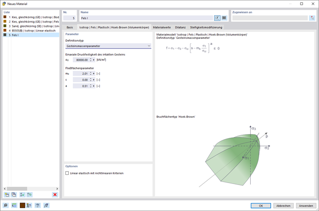
W rozszerzeniu Analiza geotechniczna dostępny jest model Hoek'a-Brown'a. Model wykazuje zachowanie materiału liniowo-sprężystego idealnie plastycznego. Jego nieliniowe kryterium wytrzymałości jest najczęściej stosowanym kryterium zniszczenia skał.
Parametry materiału można wprowadzić bezpośrednio za pomocą
- parametrów skały lub alternatywnie poprzez
- klasyfikację GSI.
opisane.
Weiterführende Informationen zu diesem Materialmodell und der Definition der Eingabe in RFEM finden Sie im entsprechenden Kapitel im Online-Handbuch für das Add-On Geotechnische Analyse: Model Hoeka-Browna .
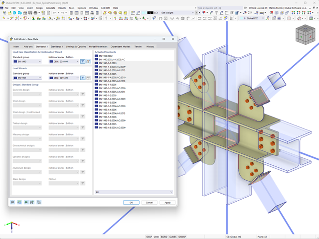
Parametry załączników krajowych (NA) do Eurokodu 3 z następujących krajów są zintegrowane:
-
 DIN EN 1993-1-1/NA:2016-04 (Niemcy)
 -
 ÖNORM EN 1993-1-1/NA:2015-12 (Austria)
 -
 SN EN 1993-1-1/NA:2016-07 (Szwajcaria)
 -
 BDS EN 1993-1-1/NA:2015-10 (Bułgaria)
 -
 BS EN 1993-1-1/NA:2016-07 (Wielka Brytania)
 -
 CEN EN 1993-1-1/2015-06 (Unia Europejska)
 -
 CYS EN 1993-1-1/NA:2015-07 (Cypr)
 -
 CSN EN 1993-1-1/NA:2016-06 (Republika Czeska)
 -
 DS EN 1993-1-1/NA:2015-07 (Dania)
 -
 ELOT EN 1993-1-1/NA:2017-01 (Grecja)
 -
 EVS EN 1993-1-1/NA:2015-08 (Estonia)
 -
 HRN EN 1993-1-1/NA:2016-03 (Chorwacja)
 -
 I S. EN 1993-1-1/NA:2016-03 (Irlandia)
 -
 ILNAS EN 1993-1-1/NA:2015-06 (Luksemburg)
 -
 IST EN 1993-1-1/NA:2015-11 (Islandia)
 -
 LST EN 1993-1-1/NA:2017-01 (Litwa)
 -
 LVS EN 1993-1-1/NA:2015-10 (Łotwa)
 -
 MS EN 1993-1-1/NA:2010-01 (Malezja)
 -
 MSZ EN 1993-1-1/NA:2015-11 (Węgry)
 -
 NBN EN 1993-1-1/NA:2015-07 (Belgia)
 -
 NEN EN 1993-1-1/NA:2016-12 (Holandia)
 -
 NF EN 1993-1-1/NA:2016-02 (Francja)
 -
 NP EN 1993-1-1/NA:2009-03 (Portugalia)
 -
 NS EN 1993-1-1/NA:2015-09 (Norwegia)
 -
 PN EN 1993-1-1/NA:2015-08 (Polska)
 -
 SFS EN 1993-1-1/NA:2015-08 (Finlandia)
 -
 SIST EN 1993-1-1/NA:2016-09 (Słowenia)
 -
 SR EN 1993-1-1/NA:2016-04 (Rumunia)
 -
 SS EN 1993-1-1/NA:2019-05 (Singapur)
 -
 SS EN 1993-1-1/NA:2015-06 (Szwecja)
 -
 STN EN 1993-1-1/NA:2015-10 (Słowacja)
 -
 TKP EN 1993-1-1/NA:2015-04 (Białoruś)
 -
 UNE EN 1993-1-1/NA:2016-02 (Hiszpania)
 -
 UNI EN 1993-1-1/NA:2015-08 (Włochy)

W rozszerzeniu Połączenia stalowe można zdefiniować kilka żeber jednocześnie na jednym pręcie lub płycie. Układ może być zdefiniowany według układu ortogonalnego lub biegunowego.
- 002801
- Ogólne informacje
- Projektowanie konstrukcji betonowych RFEM 6
- Projektowanie konstrukcji betonowych RSTAB 9
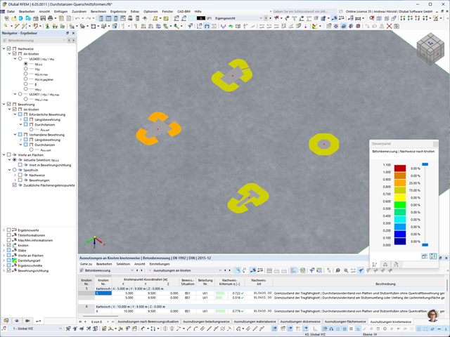
Masz indywidualne przekroje słupów i ścian o różnej geometrii, które wymagają obliczenia nośności na przebicie?
Nie ma problemu. W programie RFEM 6 można przeprowadzić obliczenia na przebicie nie tylko dla przekrojów prostokątnych i okrągłych, ale także dla dowolnego kształtu przekroju.
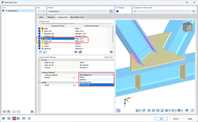
Za pomocą komponentu "Cięcie płyty" można ciąć blachy (np. blachy węzłowe, blachy środnika itp.). Dostępne są różne metody cięcia:
- Płaszczyzna: Cięcie jest wykonywane na powierzchni najbliższej płycie odniesienia.
- Powierzchnia: Wycinane są tylko przecinające się części płyt.
- Bryła ograniczająca: Najbardziej zewnętrzny wymiar, szerokość i wysokość, jest wycinany jako prostokąt.
- Otoczka wypukła: Zewnętrzna otoczka przekroju służy do przycinania płyty. Jeżeli w węzłach narożnych przekroju występują zaokrąglenia, cięcie jest do nich dostosowywane.
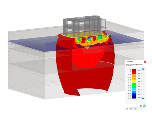
- Realistyczne odwzorowanie interakcji między budynkiem a gruntem
- Realistyczne odwzorowanie oddziaływania poszczególnych fundamentów na siebie nawzajem
- Biblioteka parametrów gruntowych z możliwością rozszerzania
- Możliwość uwzględniania wielu próbek gruntu z różnych lokalizacji, także poza obrysem budynku
- Określanie osiadań oraz wykresów naprężeń w gruncie oraz ich prezentacja w formie graficznej i tabelarycznej
_(1).png?mw=640&hash=415f7bbaf70e41679bb0106e1cf91eaa8c493ec9)
- Automatyczne generowanie modeli do analizy ES: rozszerzenie automatycznie tworzy w tle model elementów skończonych (ES) połączenia stalowego.
- Uwzględnienie wszystkich sił wewnętrznych: Obliczenia obejmują wszystkie siły wewnętrzne (N , Vy, Vz ,My, Mz, MT ) i nie są ograniczone do obciążeń płaskich.
- Automatyczne przenoszenie obciążeń: Wszystkie kombinacje obciążeń są automatycznie przenoszone do modelu analitycznego ES połączenia. Obciążenia są przenoszone bezpośrednio z programu RFEM, dzięki czemu ręczne wprowadzanie danych nie jest konieczne.
- Wydajne modelowanie: Rozszerzenie pozwala zaoszczędzić czas podczas modelowania złożonych sytuacji związanych z połączeniami. Utworzony model analityczny ES można również zapisać i wykorzystać do własnych szczegółowych analiz.
- Rozszerzalna biblioteka: Dostępna jest obszerna, rozszerzalna biblioteka zawierająca wstępnie zdefiniowane szablony połączeń stalowych.
- Szerokie zastosowanie: Rozszerzenie jest odpowiednie do tworzenia połączeń każdego typu i kształtu, jest kompatybilne z prawie wszystkimi przekrojami walcowanymi, spawanymi, złożonymi i cienkościennymi.

- 002109
- Ogólne informacje
- Optymalizacja i koszty | Szacowanie emisji CO2 RFEM 6
- Optymalizacja i koszty | Szacowanie emisji CO2 RSTAB 9
Masz pytania dotyczące programu? Optymalizacja konstrukcji w programach RFEM i RSTAB jest uzupełnieniem parametrycznego wprowadzania danych. Jest to proces równoległy, niezależny od rzeczywistych obliczeń modelu wraz ze wszystkimi jego zwykłymi definicjami obliczeń i obliczeń. Rozszerzenie zakłada, że model lub blok jest zbudowany w kontekście parametrycznym i jest kontrolowany przez globalne parametry kontrolne typu "optymalizacja". Dlatego te parametry kontrolne mają dolną i górną granicę oraz wielkość kroku w celu ograniczenia zakresu optymalizacji. Aby znaleźć optymalne wartości parametrów kontrolnych, należy określić kryterium optymalizacji (na przykład minimalny ciężar) przy wyborze metody optymalizacji (na przykład optymalizacja roju cząstek).
Oszacowanie kosztów i emisji CO2 można znaleźć już w definicjach materiałów. Obie opcje można aktywować osobno w każdej definicji materiału. Oszacowanie oparte jest na koszcie jednostkowym lub jednostkowej wartości emisji dla prętów, powierzchni oraz brył. W tym przypadku można wybrać, czy jednostki mają zostać podane według masy, objętości czy powierzchni.
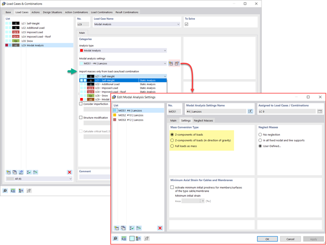
Dostępnych jest kilka opcji definiowania mas dla analizy modalnej. Masy od ciężaru własnego są uwzględniane automatycznie, natomiast obciążenia i masy można uwzględnić bezpośrednio w przypadku obciążenia typu analiza modalna. Potrzebujesz więcej opcji? Należy wybrać, czy obciążenia pełne mają być uwzględniane jako masy, składowe obciążenia w globalnym kierunku Z, czy tylko składowe obciążenia w kierunku siły ciężkości.
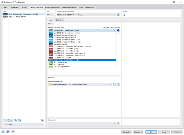
Program oferuje dodatkową lub alternatywną opcję importu mas: Ręczna definicja kombinacji obciążeń, począwszy od których masy są uwzględniane w analizie modalnej. Wybrałeś normę obliczeniową? Następnie można utworzyć sytuację obliczeniową typu Kombinacja mas sejsmicznych. W ten sposób program automatycznie oblicza sytuację masową dla analizy modalnej zgodnie z preferowaną normą obliczeniową. Innymi słowy: Program tworzy kombinację obciążeń na podstawie współczynników kombinacji wstępnie ustawionych dla wybranej normy. Zawiera on masy użyte do analizy modalnej.

W przypadku analizy spektrum odpowiedzi modeli budynków można wyświetlić współczynniki wrażliwości dla kierunków poziomych według kondygnacji.
Dzięki tym kluczowym wartościom można zinterpretować wrażliwość na efekty stateczności.

- 002108
- Ogólne informacje
- Optymalizacja i koszty | Szacowanie emisji CO2 RFEM 6
- Optymalizacja i koszty | Szacowanie emisji CO2 RSTAB 9
- Technologia sztucznej inteligencji (AI): Optymalizacja roju cząstek (PSO)
- Optymalizacja konstrukcji ze względu na minimalny ciężar lub deformację
- Możliwość zastosowania dowolnej liczby parametrów optymalizacyjnych
- Określanie zakresów zmiennych
- Optymalizacja przekrojów i materiałów
- Typy definicji parametrów
- Optymalizacja | Rosnąco, czyli optymalizacja | Malejąca
- Zastosowanie parametrycznych modeli i bloków
- Parametryzacja bloków w języku JavaScript na podstawie kodu
- Optymalizacja z uwzględnieniem wyników obliczeń
- Tabelaryczne przedstawienie najlepszych mutacji modelu
- Wyświetlanie w czasie rzeczywistym mutacji modelu w procesie optymalizacji
- Kalkulacja kosztów modelu dzięki zadanym cenom jednostkowym
- Określanie potencjału tworzenia efektu cieplarnianego (GWP-global warming potential) na etapie tworzenia modelu poprzez szacowanie równoważnej emisji CO2
- Określanie jednostkowych wskaźników zależnych od masy, objętości i powierzchni (cena i emisja CO2)
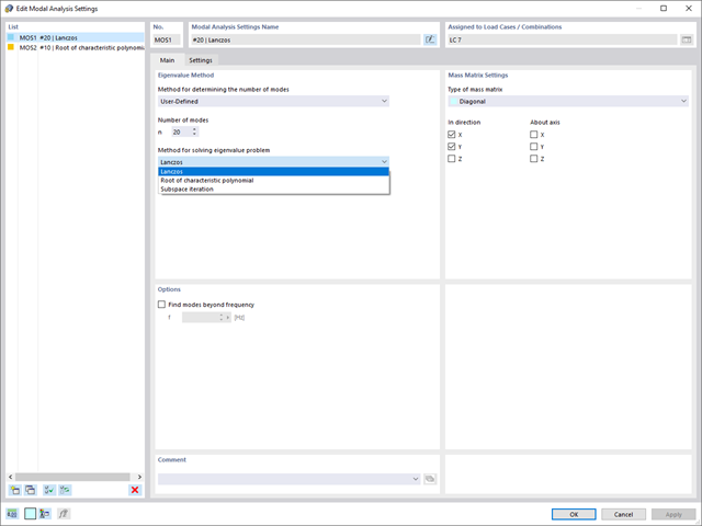
W programie RFEM dostępne są trzy wydajne solwery wartości własnych:
- pierwiastek wielomianu charakterystycznego
- Metoda Lanchosa
- iteracja podprzestrzeni
Z kolei program RSTAB oferuje dwa solwery wartości własnych:
- iteracja podprzestrzeni
- Metoda Powera z przesuniętą odwrotnością
Wybór solwera wartości własnych zależy przede wszystkim od rozmiaru modelu.

W rozszerzeniu Projektowanie konstrukcji betonowych można zdefiniować istniejące pionowe zbrojenie na ścinanie. Jest to następnie uwzględniane przy obliczaniu wytrzymałości na przebicie.

- 002110
- Ogólne informacje
- Optymalizacja i koszty | Szacowanie emisji CO2 RFEM 6
- Optymalizacja i koszty | Szacowanie emisji CO2 RSTAB 9
Istnieją dwie metody optymalizacji, dzięki którym można znaleźć optymalne wartości parametrów według kryterium ciężaru lub odkształcenia.
Najbardziej wydajną metodą o najkrótszym czasie obliczeń jest optymalizacja roju cząstek zbliżona do naturalnej (PSO). Czy słyszałeś lub czytałeś o tym? Ta technologia sztucznej inteligencji (AI) ma silną analogię do zachowania stad zwierząt szukających miejsca odpoczynku. W takich rojach można znaleźć wiele osób (por. rozwiązanie optymalizacyjne - na przykład waga), które lubią przebywać w grupie i podążać za ruchem grupy. Załóżmy, że każdy pręt roju musi zostać poddany spoczynkowi w optymalnym miejscu (por. najlepsze rozwiązanie - na przykład najniższa waga). Potrzeba ta wzrasta wraz ze zbliżaniem się do miejsca odpoczynku. Na zachowanie roju mają zatem wpływ również właściwości przestrzeni (por. wykres wyników).
Dlaczego wycieczka do biologii? Po prostu - proces PSO w RFEM lub RSTAB przebiega w podobny sposób. Proces obliczeń rozpoczyna się od wyniku optymalizacji poprzez losowe przypisanie parametrów, które mają zostać zoptymalizowane. Wielokrotnie określa nowe wyniki optymalizacji ze zróżnicowanymi wartościami parametrów, które opierają się na doświadczeniach z wcześniej przeprowadzonych mutacji modelu. Proces jest kontynuowany do momentu osiągnięcia określonej liczby możliwych mutacji modelu.
Jako alternatywa dla tej metody program oferuje również metodę przetwarzania wsadowego. Metoda ta ma na celu sprawdzenie wszystkich możliwych mutacji modelu poprzez losowe określanie wartości parametrów optymalizacji, aż do osiągnięcia określonej liczby możliwych mutacji modelu.
Po obliczeniu mutacji modelu obydwa warianty sprawdzają również odpowiednie aktywowane wyniki obliczeń rozszerzeń. Ponadto zapisuje on wariant z odpowiednim wynikiem optymalizacji i przypisaniem wartości parametrów optymalizacji, jeżeli wykorzystanie jest < 1.
Na podstawie odpowiednich sum poszczególnych materiałów można określić szacunkowe koszty całkowite i emisję. Na sumę materiałów składają się zależne od ciężaru, objętości i powierzchnie elementów prętowych, powierzchniowych i bryłowych.
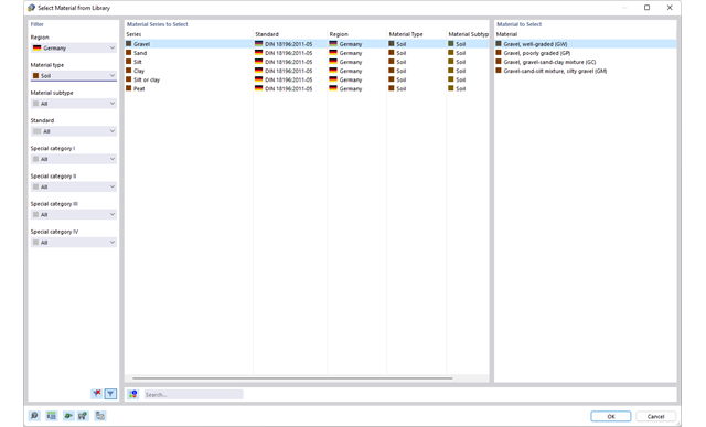
Wprowadzenie i modelowanie bryły gruntowej bezpośrednio w programie RFEM. Modele materiałów gruntowych można łączyć ze wszystkimi popularnymi rozszerzeniami dla programu RFEM.
Umożliwia to łatwą analizę całych modeli z pełną prezentacją interakcji grunt-konstrukcja.
Wszystkie parametry wymagane do obliczeń są określane automatycznie na podstawie wprowadzonych danych materiałowych. Następnie program generuje krzywe naprężenie-odkształcenie dla każdego elementu ES.
- Automatyczne uwzględnianie masy własnej od ciężaru konstrukcji
- Możliwy bezpośredni import mas z przypadków obciążeń lub kombinacji
- Opcjonalne definiowanie mas dodatkowych (masy węzłowe, liniowe lub powierzchniowe oraz masy wynikające z bezwładności) bezpośrednio w przypadkach obciążeń
- Opcjonalne pominięcie mas (na przykład masy fundamentów)
- Kombinacje mas w różnych przypadkach i kombinacjach obciążeń
- Predefiniowane współczynniki kombinacji wg różnych norm (EC 8, SIA 261, ASCE 7, ...)
- Opcjonalny import stanów początkowych (np. w celu uwzględnienia naprężenia wstępnego i imperfekcji)
- modyfikacja konstrukcji
- Uwzględnianie uszkodzenia w podporach lub prętach/powierzchniach/bryłach
- Możliwość zadania kilku analiz modalnych (np. w celu analizy różnych mas lub modyfikacji sztywności)
- Wybór typu macierzy mas (macierz diagonalna, macierz spójna, macierz jednostkowa) oraz wskazanych przez użytkownika stopni swobody (translacyjne i rotacyjne)
- Metody określania liczby postaci drgań własnych (liczba zdefiniowana przez użytkownika, liczba określana automatycznie - w celu osiągnięcia zadanych efektywnych współczynników masy modalnej, liczba określana automatycznie - w celu osiągnięcia maksymalnej częstotliwości drgań własnych - dostępne tylko w programie RSTAB)
- Określanie postaci drgań i mas w węzłach siatki MES
- Wyniki w postaci wartości własnych, częstości kątowych, częstotliwości drgań własnych i okresu drgań własnych
- Wyniki w postaci mas modalnych, efektywnych mas modalnych, współczynników masy modalnej i współczynników udziału masy
- Tabelaryczne i graficzne przedstawienie mas w punktach siatki MES
- Wizualizacja i animacja postaci drgań własnych
- Różne opcje skalowania postaci drgań własnych
- Dokumentacja wyników numerycznych i graficznych w raporcie
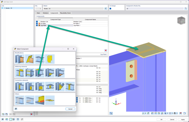
Teraz za pomocą kilku kliknięć można wstawiać blachy czołowe w połączeniach stalowych. Dane można wprowadzać za pomocą znanych typów definicji 'Offset' lub 'Wymiary i położenie'. Wprowadzając pręt odniesienia i płaszczyznę cięcia, można również pominąć część Przekrój pręta.
Za pomocą tego komponentu można łatwo modelować na przykład blachy czołowe na końcach słupa.
W ustawieniach analizy modalnej należy wprowadzić wszystkie dane, które są niezbędne do określenia częstotliwości drgań własnych. Są to na przykład kształty mas i solwery wartości własnych.
Rozszerzenie Analiza modalna określa najniższe wartości częstości drgań własnych konstrukcji. Liczbę wartości własnych można dostosować lub określić automatycznie. Należy zatem osiągnąć efektywne współczynniki masy modalnej lub maksymalne częstotliwości drgań własnych. Masy są importowane bezpośrednio z przypadków obciążeń i kombinacji obciążeń. W takim przypadku istnieje możliwość uwzględnienia masy całkowitej, składowych obciążenia w globalnym kierunku Z lub tylko składowej obciążenia w kierunku siły ciężkości.
Dodatkowe masy w węzłach, liniach, prętach lub powierzchniach można zdefiniować ręcznie. Ponadto można wpływać na macierz sztywności poprzez import sił osiowych lub modyfikacji sztywności z przypadku obciążenia lub kombinacji obciążeń.
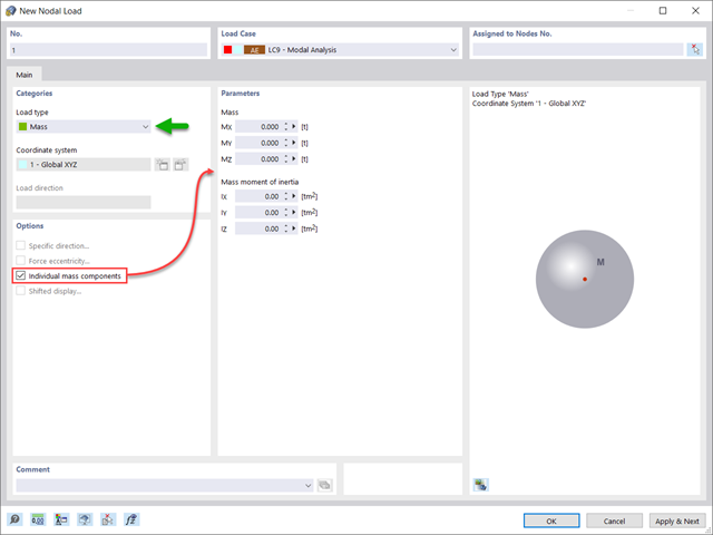
Czy oprócz obciążeń statycznych chcesz uwzględnić również inne obciążenia jako masy? Program umożliwia to dla obciążeń węzłowych, prętowych, liniowych i powierzchniowych. W tym celu podczas definiowania obciążenia należy wybrać typ Obciążenie masą. Dla takich obciążeń należy zdefiniować masę lub składowe masy w kierunkach X, Y i Z. W przypadku mas węzłowych można dodatkowo zdefiniować momenty bezwładności X, Y i Z w celu modelowania bardziej złożonych punktów mas.