


General
Simulations performed using the finite element method are based on what is known as discretization. In this case, a problem with an unknown solution is decomposed into sub-problems for which an approximate solution can be determined. In the present case, this is a geometric decomposition into finite (finite) components (elements) whose physical behavior can be approximately described by approximation functions. This leads to the importance of performing a mesh convergence study. The FE mesh is usually refined iteratively, starting from a coarse mesh. The goal of such a study is to select a mesh that provides sufficiently accurate results. A middle way is sought. On one hand, the mesh should be fine enough that additional refinement does not result in any further relevant increase in accuracy, but on the other hand, it should be as rough as possible in order to conserve resources (computing time/memory space). Reaching the convergence limit, e.g. less than 1% change in the results between the steps, indicates a stable solution. In general, convergence is more likely to be achieved for displacements than for higher-order results, such as stresses and strains. It is important to select a special point for monitoring, because the change of the mesh can also lead to a change of the coordinates of the FE mesh nodes. In RFEM, you can achieve this, for example, by evaluating geometrically defined nodes or by using additional surface result points.
You can control the meshing in RFEM using various mesh settings. It may be advisable not to refine the entire model if the results depend on the local mesh. For this purpose, RFEM provides the option of local FE mesh refinement.
Example of Deflection on Cantilever
As mentioned above, the easiest way to achieve convergence is by looking at the deformations. In the following, you can see an example according to Bernd Klein [1] that examines the influence of meshing on the final displacement of a cantilever. The model consists of an aluminum cantilever with a length of 100 mm and a modulus of elasticity of 70 GPa. The cross-section is a flat upright plate with a height of 20 mm and a width of 1 mm. A load of 1 kN is applied at the end of the cantilever.

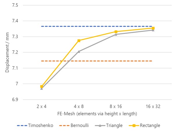
The goal is to study the deformation at the end of the cantilever, which was modeled using surfaces, as a function of mesh density. In addition, different meshing types, triangular and quadrilateral elements, were analyzed. For comparison, the modeling was also carried out using beam elements, with (Timoshenko) and without (Bernoulli), considering the shear strain. The model of beam and quadrangle elements, as well as the results obtained, are shown in the image below.

As you can see, the meshing of the beam element has no influence on the deformation of the end node in this case. However, the shear strain is considered, as expected. The deformation without shear distortion (Bernoulli) is lower, at 7.145 mm, than according to Timoshenko, at 7.365 mm. The deformations of the cantilever surfaces approach this value as the meshing refinement increases. These relations are clearly visible in the following diagram.
Example of Stress and Strain on Plate
The next example shows the influence of the meshing on the calculated stress and strain results. For this purpose, a surface was modeled with a free rectangular load and lifting line supports.

The meshing convergence is checked at a surface result point located at a corner of the free rectangular load. The following image illustrates this principle. The upper window shows the model with meshing, the middle window shows the first principal stresses obtained, and the lower one shows those of the first principal strains. The meshing increases in the models from left to right.

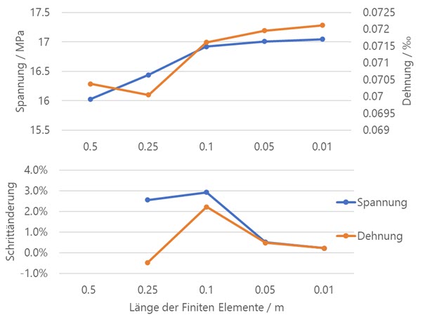
The following diagram shows the approximation of the stress and strain values with increasing mesh fineness to a limit value, known as convergence behavior. As it is not easy to determine the actual value of the stress here, it is advisable to evaluate the relative change compared to the previous meshing step. This is shown in the lower part of the diagram. With a target FE element length of 0.01 m, both stress and strain deviate by only about 0.2% from the previous refinement step.
Example: Linear Buckling Analysis of Cylindrical Shell
When determining the eigenvalues, the mesh refinement is also expected to have a significant influence. On the one hand, this affects the number of mode shapes, which depends directly on the degrees of freedom. On the other hand, local stiffening effects and the distribution of mass points are also relevant. For this reason, a mesh convergence check should also be performed for stability analyses and dynamic simulations, specifically modal analyses.
The following example is inspired by a paper by Łukasz Skotny, Ph.D. [2] and was first published by Ondřej Švorc on LinkedIn. The model consists of a 0.2 m high, 2 mm thick aluminum cylindrical shell (EN AW-3004 H14) with a diameter of 0.1 m. The top and bottom surfaces are modeled as rigid surfaces and are loaded with 1 kN, respectively, or supported in place. By successively refining the mesh from 15 mm to 3 mm, the influence of mesh refinement on the critical load of the linear buckling analysis is analyzed.

The following image displays the results of the buckling analysis for an FE mesh length of 15, 6, and 3 mm with a deformed mesh.

The ideal critical load for this case can also be determined analytically according to EN 1999-1-5, based on the classical shell theory by Lorenz/Timoshenko/Southwell. The calculation for a long cylinder, with verification of the slenderness limit, is shown in the following formula:
The mesh convergence study showed that the critical load decreases with increasing mesh refinement and approaches a limit value. The following diagram shows the critical load as a function of the number of elements (left) and their reciprocal (right). The coarsest mesh (15 mm) thus overestimates the critical load by approximately 25.5%. The critical load of the finest mesh is 1008 kN, which is approximately 5.3% below the analytically determined value. Possible reasons for this include the influence of the boundary conditions as well as the stiffness behavior of the shell elements implemented in RFEM.

The following image displays the deviation of the critical load from the result of the finest mesh analyzed as a function of the calculation time (left) and the mesh size (right). Starting at a mesh size of 5 mm, the relative change compared to the next coarser step is less than 2%, as is the case with the result of the finest mesh (3 mm). The calculation time, however, nearly triples from approximately 11 to 30 s. This relation shows the compromise between calculation time and accuracy, which is typical for FE simulations.

Analytical and standard-compliant limits for mesh refinement can also be found for this example. According to EN 1993-1-6:2007 Annex §C.3, it is necessary to perform a convergence study with at least 3 mesh levels and a refinement factor greater than or equal to 1.5. The convergence criterion here is a change in αcr of less than or equal to 1% between the last two levels. According to prEN 1993-1-14 §4, which has not yet been introduced, the mesh must be able to resolve the governing failure mode. For buckling analyses, this is the critical buckling half-wave length. For good resolution, 4 elements can be assumed to be sufficient here. The mesh size for this geometry is thus approximately 4 mm. This also agrees with the results of the convergence study performed here (relative change ~ 1%).
It should also be noted in this case that a mesh that is too fine is not automatically better. With very small elements, the condition number of the stiffness matrix increases, which can lead to numerical inaccuracies in the eigenvalue solver (Lanczos, subspace iteration). The optimal value is a sharply resolved buckling mode with a mesh size of approximately 3.5 mm.
Final Notes
The examples selected here are intended to show a simplified procedure for the mesh convergence study. However, it should be noted that other parameters may be the target of this investigation in individual simulations. Furthermore, different factors may lead to different requirements. These can be of a geometric nature, for example, where a curvature needs to be represented very accurately by the elements. Also, the analysis of local damage (for example, brittle failure behavior) requires a comparatively finer mesh than for plastification.
If there is no approximation to a limit value with increasing mesh refinement, this could be a singularity problem. You can find more information about this in the technical article at the following link.