78 Results
View Results:
Sort by:
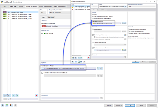
To evaluate whether it is also necessary to consider the second-order analysis in a dynamic calculation, the sensitivity coefficient of interstory drift θ is provided in EN 1998‑1, Sections 2.2.2 and 4.4.2.2. It can be calculated and analyzed using RFEM 6 and RSTAB 9.
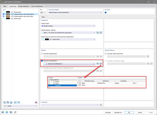
Both the determination of natural vibrations and the response spectrum analysis are always performed on a linear system. If nonlinearities exist in the system, they are linearized and thus not taken into account. They are caused by, for example, tension members, nonlinear supports, or nonlinear hinges. This article shows how you can handle them in a dynamic analysis.
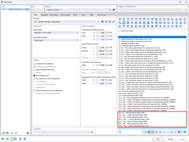
To be able to evaluate the influence of local stability phenomena of slender structural components, RFEM 6 and RSTAB 9 provide you with the option of performing a linear critical load analysis on the cross-section level. The following article explains the basics of the calculation and the result interpretation.
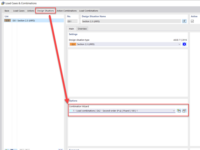
The CSA S16:19 Stability Effects in Elastic Analysis method in Annex O.2 is an alternative option to the Simplified Stability Analysis Method in Clause 8.4.3. This article will describe the requirements of Annex O.2 and application in RFEM 6.
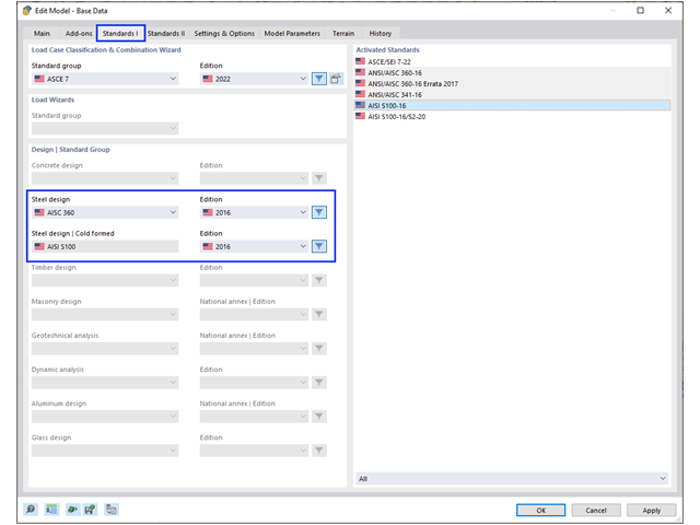
The design of cold-formed steel members according to the AISI S100-16 is now available in RFEM 6. Design can be accessed by selecting “AISC 360” as the standard in the Steel Design add-on. “AISI S100” is then automatically selected for the cold-formed design (Image 01).
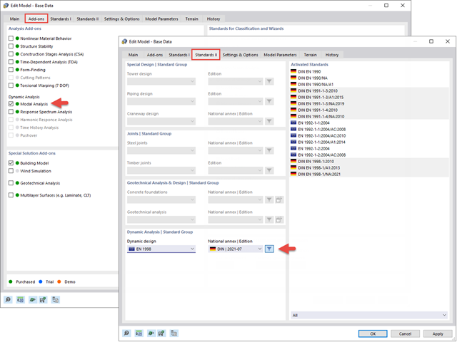
Modal analysis is the starting point for the dynamic analysis of structural systems. You can use it to determine natural vibration values such as natural frequencies, mode shapes, modal masses, and effective modal mass factors. This outcome can be used for vibration design, and it can be used for further dynamic analyses (for example, loading by a response spectrum).
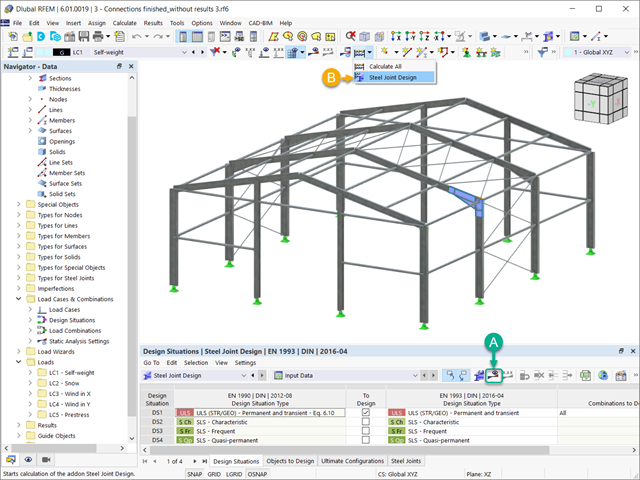
The advantage of the RFEM 6 Steel Joints add-on is that you can analyze steel connections using an FE model for which the modeling runs fully automatically in the background. The input of the steel joint components that control the modeling can be done by defining the components manually, or by using the available templates in the library. The latter method is included in a previous Knowledge Base article titled “Defining Steel Joint Components Using the Library". The definition of parameters for the design of steel joints is the topic of the Knowledge Base article “Designing Steel Joints in RFEM 6".
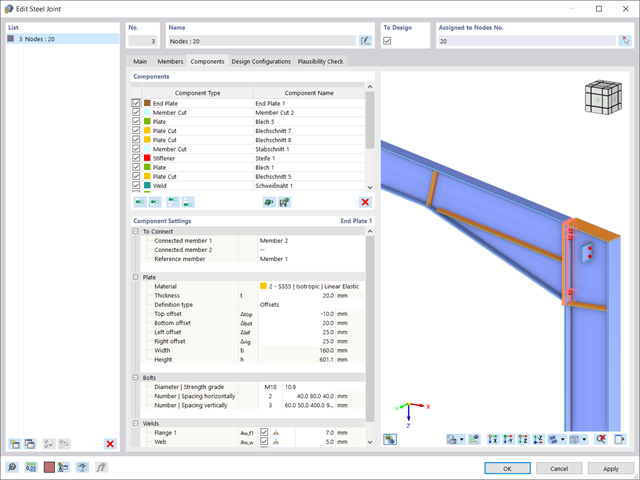
Steel connections in RFEM 6 are defined as an assembly of components. In the new Steel Joints add-on, universally applicable basic components (plates, welds, auxiliary planes) are available for entering complex connection situations. The methods with which connections can be defined are considered in two previous Knowledge Base articles: “A Novel Approach to Designing Steel Joints in RFEM 6" and “Defining Steel Joint Components Using the Library".
In accordance with Sect. 6.6.3.1.1 and Clause 10.14.1.2 of ACI 318-19 and CSA A23.3-19, respectively, RFEM effectively takes into consideration concrete member and surface stiffness reduction for various element types. Available selection types include cracked and uncracked walls, flat plates and slabs, beams, and columns. The multiplier factors available within the program are taken directly from Table 6.6.3.1.1(a) and Table 10.14.1.2.
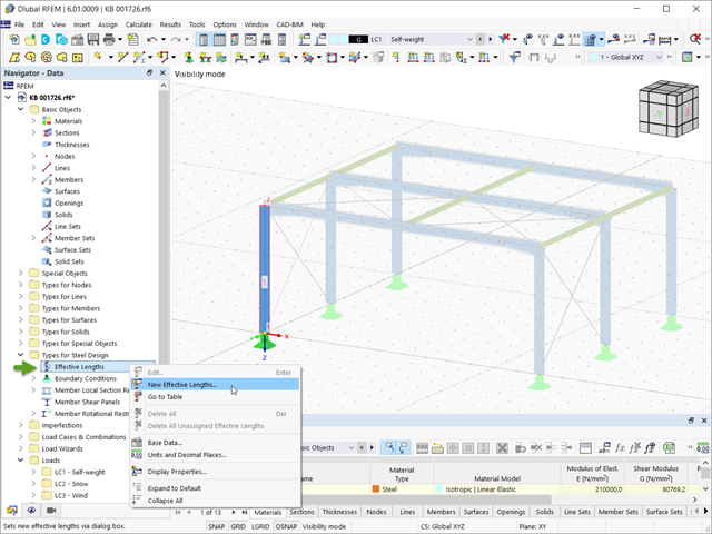
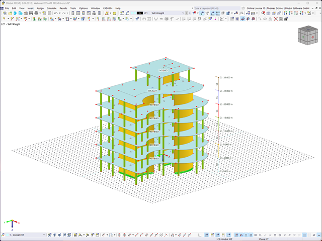
The stability checks for the equivalent member design according to EN 1993-1-1, AISC 360, CSA S16, and other international standards require consideration of the design length (that is, the effective length of the members). In RFEM 6, it is possible to determine the effective length manually by assigning nodal supports and effective length factors or, on the other hand, by importing it from the stability analysis. Both options will be demonstrated in this article by determining the effective length of the framed column in Image 1.