
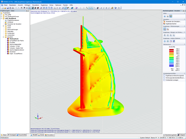
In RFEM and RSTAB, you can visualize the flow field quantities of pressure, velocity, turbulence kinetic energy, and turbulence dissipation rate for the wind simulation.
The clipping planes are aligned with the respective wind direction.
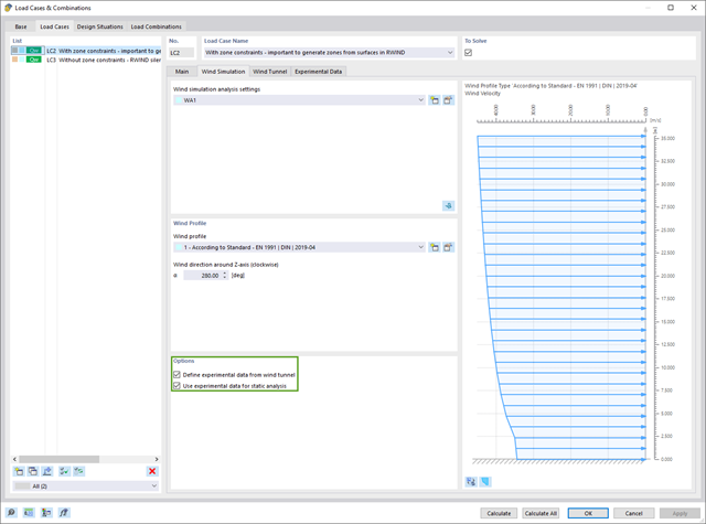
If you have experimentally determined surface pressures available for a model, you can apply them to a structural model in RFEM 6, process them in RWIND 2, and use them as wind loads in the structural analysis of RFEM 6.
You can find out how to apply the experimentally determined values in this technical article.

The modal relevance factor (MRF) can help you to assess to which extent specific elements participate in a specific mode shape. The calculation is based on the relative elastic deformation energy of each individual member.
The MRF can be used to distinguish between local and global mode shapes. If multiple individual members show significant MRF (for example, > 20%), the instability of the entire structure or a substructure is very likely. On the other hand, if the sum of all MRFs for an eigenmode is around 100%, a local stability phenomenon (for example, buckling of a single bar) can be expected.
Furthermore, the MRF can be used to determine critical loads and equivalent buckling lengths of certain members (for example, for stability design). Mode shapes for which a specific member has small MRF values (for example, < 20%) can be neglected in this context.
The MRF is displayed by mode shape in the result table under Stability Analysis → Results by Members → Effective Lengths and Critical Loads.
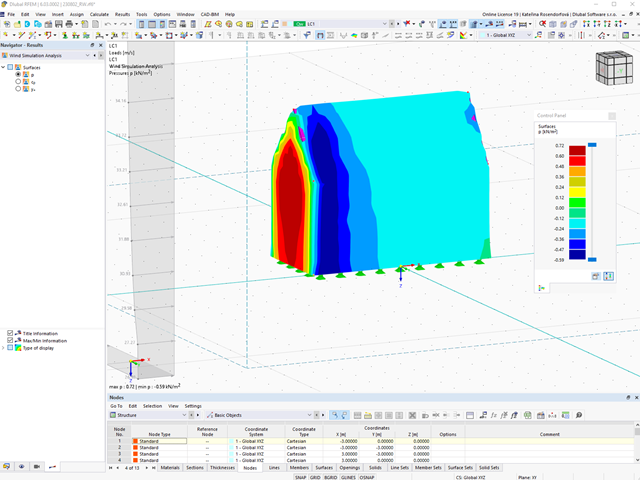
You can display the RWIND results directly in the main program. In the Navigator - Results, select the Wind Simulation Analysis result type from the list above.
Currently, the following results are available, which refer to the RWIND computational mesh:
- Surface pressure
- Surface cp coefficient
- Wall distance y+ (steady flow)
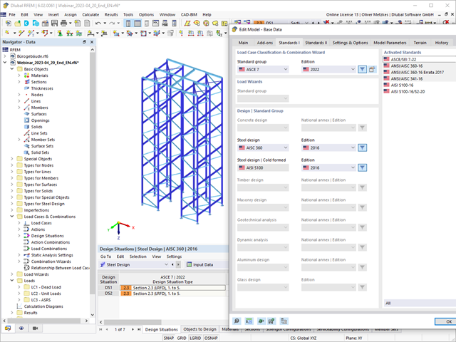
The design of cold-formed steel members according to the AISI S100-16 / CSA S136-16 is available in RFEM 6. Design can be accessed by selecting “AISC 360” or “CSA S16” as the standard in the Steel Design Add-on. “AISI S100” or “CSA S136” is then automatically selected for the cold-formed design.
RFEM applies the Direct Strength Method (DSM) to calculate the elastic buckling load of the member. The Direct Strength Method offers two types of solutions, numerical (Finite Strip Method) and analytical (Specification). The FSM signature curve and buckling shapes can be viewed under Sections.
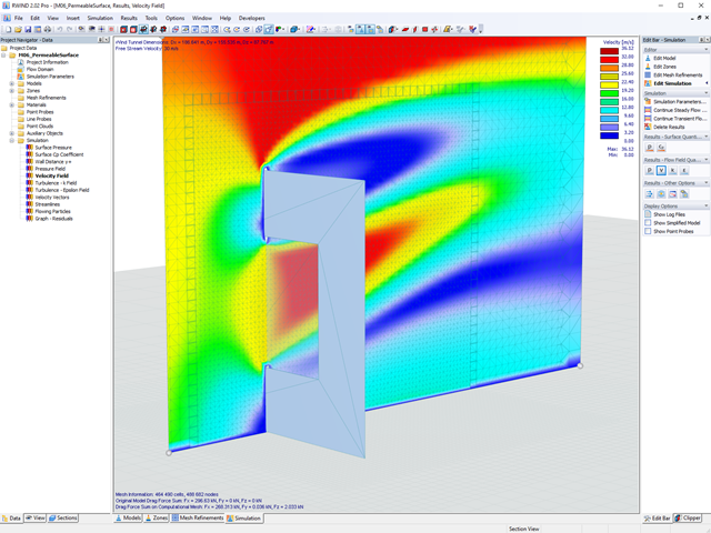
Use RWIND 2 Pro to easily apply a permeability to a surface. All you need is the definition of
- the Darcy coefficient D,
- the inertial coefficient I, and
- the length of the porous medium in the direction of flow L,
to define a pressure boundary condition between the front and back of a porous zone. Due to this setting, you obtain the flow through this zone with a two-part result display on both sides of the zone area.
But that's not all. Furthermore, the generation of a simplified model recognizes permeable zones and takes into account the corresponding openings in the model coating. Can you waive an elaborate geometric modeling of the porous element? Understandable – we have good news for you then! With a pure definition of the permeability parameters, you can avoid complex geometric modeling of the porous element. Use this feature to simulate permeable scaffolding, dust curtains, mesh structures, and so on.
More Information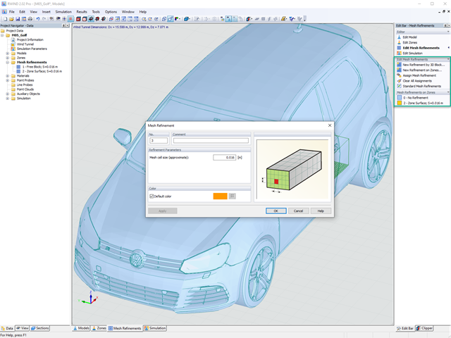
Do you already know the editor for mesh refinement control? It is a great help for your work! Why? It's easy – it gives you the following options:
- Graphic visualization of the areas with mesh refinements
- Mesh refinement of zones
- Deactivating the standard 3D solid mesh refinement with transversion into the corresponding manual 3D mesh refinements.
These options help you to formulate a suitable rule for meshing the entire model, even for the models with unusual dimensions. Use the editor to efficiently define small model details on large buildings or detailed meshing areas in the coating area of the model. You will be amazed!
.png?mw=640&hash=55038d2a1591f62179796666cb9b2fede0274e19)
A graphical and tabular output of the results for deformations, stresses, and strains helps you when determining the soil solids. To achieve this, use the special filter criteria for targeted selection of results.
The program doesn't leave you alone with the results. If you want to graphically evaluate the results in the soil solids, you can use the guide objects. For example, you can define clipping planes. This allows you to view the corresponding results in any plane of the soil solid.
And not just that. The utilization of result sections and clipping boxes facilitates the precise graphical analysis of the soil solid.
You already know that it is possible to model and analyze a soil and a structure in the entire model. As a result, you have explicitly taken into account the soil-structure interaction. By modifying a component, you achieve the immediate correct consideration in the analysis as well as in the results for the entire system of the soil and structure.

Are you ready for the evaluation? Use the calculation diagrams, which show the distribution of a specific result during the calculation.
You can freely define the layout of the vertical and horizontal axes of the calculation diagram. This allows you, for example, to consider the settlement distribution of a certain node, depending on the load.

Your data are always documented in a multilingual printout report. You can adjust the content at any time and save it as a template. You can also add graphics, texts, MathML formulas, and PDF documents to your report with just a few clicks.

Enter and model a soil solid directly in RFEM. You can combine the soil material models with all common RFEM add-ons.
This allows you to easily analyze the entire models with a complete representation of the soil-structure interaction.
All parameters required for the calculation are automatically determined from the material data that you have entered. The program then generates the stress-strain curves for each FE element.

Did you know? You can enter the soil layers that you have obtained from the subsoil expertises done in the locations into the program in the form of soil samples. Assign the explored soil materials, including their material properties, to the layers.
For the definition of the samples, you can enter the data in tables as well as in the respective editing dialog box. Furthermore, you can also specify the groundwater level in the soil samples.

The soil solids that you want to analyze are summarized in soil massifs.
Use the soil samples as a basis for a definition of the respective soil massif. This way, the program allows for user-friendly generation of the massif, including the automatic determination of the layer interfaces from the sample data, as well as the groundwater level and the boundary surface supports.
Soil massifs provide you with the option to specify a target FE mesh size independently of the global setting for the rest of the structure. You can thus consider the various requirements of the building and soil in the entire model.
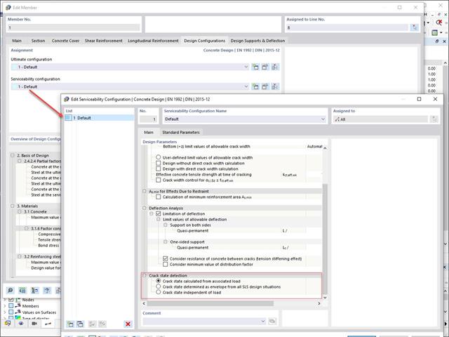
Various design parameters of the cross-sections can be adjusted in the serviceability limit state configuration. The applied cross-section condition for the deformation and crack width analysis can be controlled there.
For this, the following settings can be activated:
- Crack state calculated from associated load
- Crack state determined as an envelope from all SLS design situations
- Cracked state of cross-section - independent of load

Do you want to model and analyze the behavior of a soil solid? To ensure this, special suitable material models have been implemented in RFEM.
You can use the modified Mohr-Coulomb model with a linear-elastic ideal-plastic model or a nonlinear elastic model with an oedometric stress-strain relation. The limit criterion, which describes the transition from the elastic area to that of the plastic flow, is defined according to Mohr-Coulomb.
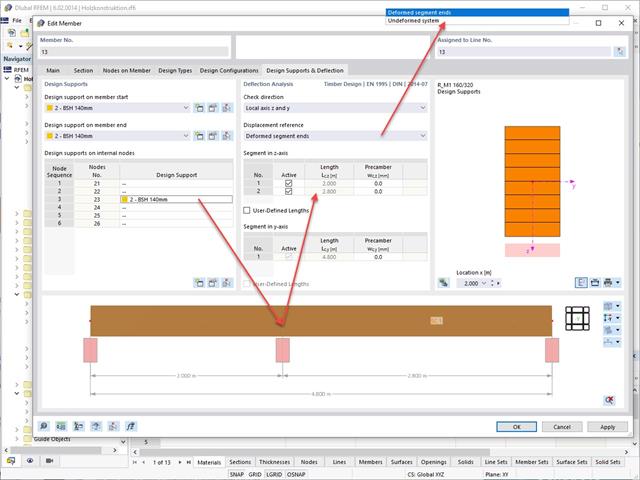
In the "Deflection and Design Support" tab under "Edit Member", the members can be clearly segmented using optimized input windows. Depending on the supports, the deformation limits for cantilever beams or single-span beams are used automatically.
By defining the design support in the corresponding direction at the member start, member end, and intermediate nodes, the program automatically recognizes the segments and segment lengths to which the allowable deformation is related. It also automatically detects whether it is a beam or a cantilever due to the defined design supports. The manual assignment, as in the previous versions (RFEM 5), is no longer necessary.
The "User-Defined Lengths" option allows you to modify the reference lengths in the table. The corresponding segment length is always used by default. If the reference length deviates from the segment length (for example, in the case of curved members), it can be adjusted.
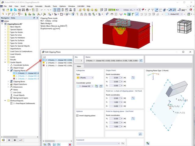
This feature also contributes to the clearly-arranged display of your results. Clipping planes are intersecting planes that you can place freely throughout the model. The zone in front of or behind the plane is consequently hidden in the display. This way, you can clearly and simply show the results in an intersection or a solid, for example.
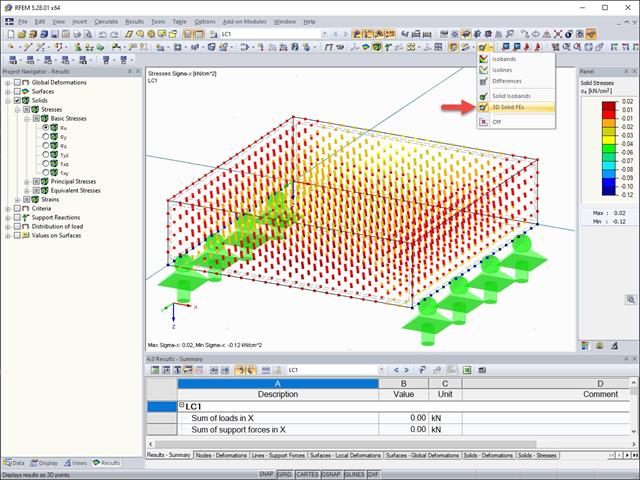
The results of solid stresses can be displayed as colored 3D points in the finite elements.

- Calculation of stationary incompressible turbulent wind flow using the SimpleFOAM solver from the OpenFOAM® software package
- Numerical scheme according to the first and second order
- Turbulence models RAS k-ω and RAS k-ε
- Consideration of surface roughness depending on model zones
- Model design via VTP, STL, OBJ, and IFC files
- Operation via bidirectional interface of RFEM or RSTAB for importing model geometries with standard-based wind loads and exporting wind load cases with probe-based printout report tables
- Intuitive model changes via drag & drop and graphical adjustment assistance
- Generation of a shrink-wrap mesh envelope around the model geometry
- Consideration of environmental objects (buildings, terrain, and so on)
- Height-dependent description of the wind load (wind speed and turbulence intensity)
- Automatic meshing depending on a selected depth of detail
- Consideration of layer meshes near the model surfaces
- Parallelized calculation with optimal utilization of all processor cores of a computer
- Graphical output of the surface results on the model surfaces (surface pressure, Cp coefficients)
- Graphical output of the flow field and vector results (pressure field, velocity field, turbulence – k-ω field, and turbulence – k-ε field, velocity vectors) on Clipper/Slicer planes
- Display of 3D wind flow via animated streamline graphics
- Definition of point and line probes
- Multilingual user interface (German, English, Czech, Spanish, French, Italian, Polish, Portuguese, Russian, and Chinese)
- Calculations of several models in one batch process
- Generator for creating rotated models to simulate different wind directions
- Optional interruption and continuation of the calculation
- Individual color panel per result graphic
- Display of diagrams with separate output of results on both sides of a surface
- Output of the dimensionless wall distance y+ in the mesh inspector details for the simplified model mesh
- Determination of the shear stress on the model surface from the flow around the model
- Calculation with an alternative convergence criterion (you can select between the residual types pressure or flow resistance in the simulation parameters)
- Calculation of transient incompressible turbulent wind flow with the BlueDyMSolver solver
- LES SpalartAllmarasDDES turbulence model
- Consideration of stationary solution as initial state for transient calculation
- Automatic determination of analysis period and time steps
- Use of intermediate results during the calculation
- Organized display of time-varying results via time step units
- Diagram of drag force and point probe results over analysis time
- Display of line probe results for any time steps in a diagram
- Freely adjustable wind permeability for surfaces (Go to Product Feature)
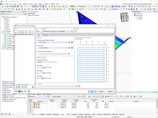
To model structures in RWIND Basic, you find a special application in RFEM and RSTAB. Here, you define the wind directions to be analyzed by means of related angular positions about the vertical model axis. At the same time, you define the elevation-dependent wind profile on the basis of a wind standard. In addition to these specifications, you can use the stored calculation parameters to determine your own load cases for a stationary calculation per each angular position.
As an alternative, you can also use the RWIND Basic program manually, without the interface application in RFEM or RSTAB. In this case, RWIND Basic models the structures and terrain environment directly from the imported VTP, STL, OBJ, and IFC files. You can define the height-dependent wind load and other fluid-mechanical data directly in RWIND Basic.
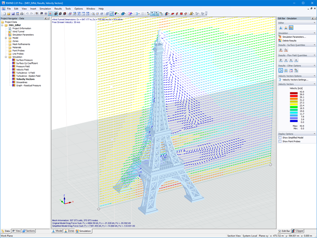
RWIND Basic uses a numerical CFD model (Computational Fluid Dynamics) to simulate wind flows around your objects using a digital wind tunnel. The simulation process determines specific wind loads acting on your model surfaces from the flow result around the model.
A 3D volume mesh is responsible for the simulation itself. For this, RWIND Basic performs an automatic meshing on the basis of freely definable control parameters. For the calculation of wind flows, RWIND Basic provides you with a stationary solve and RWIND Pro provides a transient solver for incompressible turbulent flows. Surface pressures resulting from the flow results are extrapolated onto the model for each time step.
By solving the numerical flow problem, you can obtain the following results on and around the model:
- Pressure on structure surface
- Coefficient Cp distribution on the structure surfaces
- Pressure field about the structure geometry
- Velocity field about the structure geometry
- Turbulence k-ω field about the structure geometry
- Turbulence k-ε field about the structure geometry
- Velocity vectors about the structure geometry
- Streamlines about the structure geometry
- Forces on member-shaped structures that were originally generated from member elements
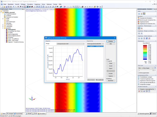
- Convergence diagram
- Direction and size of the flow resistance of the defined structures
Despite this amount of information, RWIND 2 remains clearly arranged, as is typical for the Dlubal programs. You can specify freely definable zones for a graphic evaluation. Voluminously displayed flow results about the structure geometry are often confusing – you know the problem for sure. That's why RWIND Basic provides freely movable section planes for the separate display of the "solid results" in a plane. For the 3D branched streamline result, you have an option to select between a static and an animated display in the form of moving line segments or particles. This option helps you to represent the wind flow as a dynamic effect.
You can export all results as a picture or, especially for the animated results, as a video.
When starting the analysis in the RFEM or RSTAB application, you trigger a batch process. It places all member, surface, and solid definitions of the model rotated with all relevant coefficients in the numerical wind tunnel of RWIND Basic. Furthermore, it starts the CFD analysis, and returns the resulting surface pressures for a selected time step as FE mesh nodal loads or member loads into the respective load cases of RFEM or RSTAB.
These load cases which contain RWIND Basic loads can then be calculated. Moreover, you can combine them with other loads in load and result combinations.

Compared to the RF-/STEEL Warping Torsion add-on module (RFEM 5 / RSTAB 8), the following new features have been added to the Torsional Warping (7 DOF) add-on for RFEM 6 / RSTAB 9:
- Complete integration into the environment of RFEM 6 and RSTAB 9
- 7th degree of freedom is directly taken into account in the calculation of members in RFEM/RSTAB on the entire system
- No more need to define support conditions or spring stiffnesses for calculation on the simplified equivalent system
- Combination with other add-ons is possible, for example for the calculation of critical loads for torsional buckling and lateral-torsional buckling with stability analysis
- No restriction to thin-walled steel sections (it is also possible to calculate ideal overturning moments for beams with massive timber sections, for example)

Compared to the RF‑SOILIN add-on module (RFEM‑5), the following new features have been added to the Geotechnical Analysis add-on for RFEM 6:
- Creation of the layered soil as a 3D model from the entirety of the defined soil samples
- Recognized material law according to Mohr-Coulomb for soil simulation
- Graphical and tabular output of stresses and strains at any depth of the soil
- Optimal consideration of the soil-structure interaction on the basis of an overall model

Compared to the RF‑/STABILITY (RFEM 5) and RSBUCK (RSTAB 8) add-on modules, the following new features have been added to the Structure Stability add-on for RFEM 6 / RSTAB 9:
- Activation as a property of a load case or a load combination
- Automated activation of the stability calculation via combination wizards for several load situations in one step
- Incremental load increase with user-defined termination criteria
- Modification of the mode shape normalization without recalculation
- Result tables with filter option

- Calculation of models consisting of member, shell, and solid elements
- Nonlinear stability analysis
- Optional consideration of axial forces from initial prestress
- Four equation solvers for an efficient calculation of various structural models
- Optional consideration of stiffness modifications in RFEM/RSTAB
- Determination of a stability mode greater than the user-defined load increment factor (Shift method)
- Optional determination of the mode shapes of unstable models (to identify the cause of instability)
- Visualization of the stability mode
- Basis for determining imperfection
- Consideration of 7 local deformation directions (ux, uy, uz, φx, φy, φz, ω) or 8 internal forces (N, Vu, Vv, Mt,pri, Mt,sec, Mu, Mv, Mω) when calculating member elements
- Usable in combination with a structural analysis according to linear static, second-order, and large deformation analysis (imperfections can also be taken into account)
- In combination with the Stability Analysis add-on, allows you to determine critical load factors and mode shapes of stability problems such as torsional buckling and lateral-torsional buckling
- Consideration of end plates and transverse stiffeners as warping springs when calculating I-sections with automatic determination and graphical display of the warping spring stiffness
- Graphical display of the cross-section warping of members in the deformation
- Full integration with RFEM and RSTAB