
The building model is calculated in two phases:
- Global 3D calculation of the global model, where the slabs are modeled as a rigid plane (diaphragm) or as a bending plate
- Local 2D calculation of the individual floors
After the calculation, the results of the columns and walls from the 3D calculation and the results of the slabs from the 2D calculation are combined in a single model. This means that there is no need to switch between the 3D model and the individual 2D models of the slabs. The user only works with one model, saves valuable time, and avoids possible errors in the manual data exchange between the 3D model and the individual 2D ceiling models.
The vertical surfaces in the model can be divided into shear walls and opening lintels. The program automatically generates internal result members from these wall objects, so they can be designed as members according to any standard in the Concrete Design add-on.
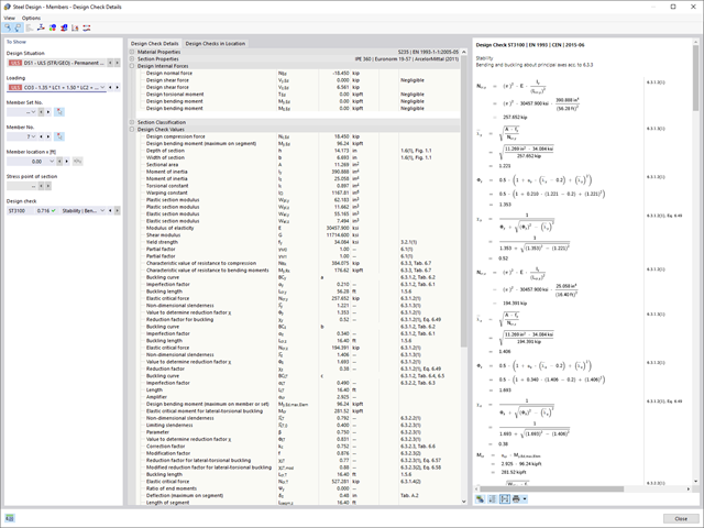
With Dlubal Software, you always have an overview, regardless of whether your projects are from the reinforced concrete, steel, timber, aluminum, or other industry. The program clearly displays the design check formulas used in your design (including a reference to the used equation from the standard). These design check formulas can also be included in the printout report.
Go to Explanatory Video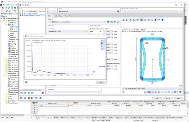
When performing a design according to EN 1993‑1‑3, it is possible to graphically display a mode shape for the distortional buckling of a cross-section, and for the RSECTION cross-sections.
The mode shape can also be output in RSECTION 1 for library cross-sections.

Have you activated the Building Model add-on? Very good! This allows you to display the center of rigidity in tabular and graphical form. Use it for your dynamic analysis, for example.
The design of cold-formed steel members according to the AISI S100-16 / CSA S136-16 is available in RFEM 6. Design can be accessed by selecting “AISC 360” or “CSA S16” as the standard in the Steel Design Add-on. “AISI S100” or “CSA S136” is then automatically selected for the cold-formed design.
RFEM applies the Direct Strength Method (DSM) to calculate the elastic buckling load of the member. The Direct Strength Method offers two types of solutions, numerical (Finite Strip Method) and analytical (Specification). The FSM signature curve and buckling shapes can be viewed under Sections.
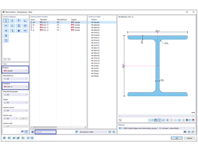
The new steel sections according to the latest CISC Handbook (12th edition) are available in RFEM 6. The sections are listed in the Standardized library. In the filter, select “Canada” for the region and “CISC 12” for the standard. Alternatively, the section name can be directly entered in the search box located at the bottom of the dialog box.

Are you ready for the evaluation? Use the calculation diagrams, which show the distribution of a specific result during the calculation.
You can freely define the layout of the vertical and horizontal axes of the calculation diagram. This allows you, for example, to consider the settlement distribution of a certain node, depending on the load.

Do you want to model and analyze the behavior of a soil solid? To ensure this, special suitable material models have been implemented in RFEM.
You can use the modified Mohr-Coulomb model with a linear-elastic ideal-plastic model or a nonlinear elastic model with an oedometric stress-strain relation. The limit criterion, which describes the transition from the elastic area to that of the plastic flow, is defined according to Mohr-Coulomb.
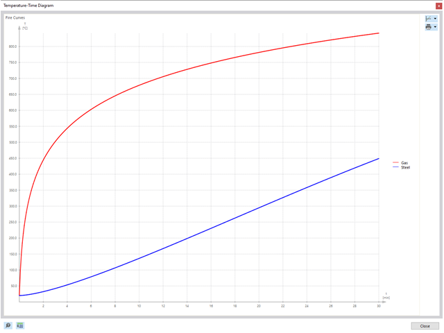
The governing component temperature at the time of analysis can be determined for the fire resistance design automatically using the input. In this case, you can follow the temperature curve in detail as a function of timeby displaying the temperature-time diagram.

Compared to the RF‑SOILIN add-on module (RFEM‑5), the following new features have been added to the Geotechnical Analysis add-on for RFEM 6:
- Creation of the layered soil as a 3D model from the entirety of the defined soil samples
- Recognized material law according to Mohr-Coulomb for soil simulation
- Graphical and tabular output of stresses and strains at any depth of the soil
- Optimal consideration of the soil-structure interaction on the basis of an overall model
Compared to the RF‑/STEEL EC3 add-on module (RFEM 5 / RSTAB 8), the following new features have been added to the Steel Design add-on for RFEM 6 / RSTAB 9:
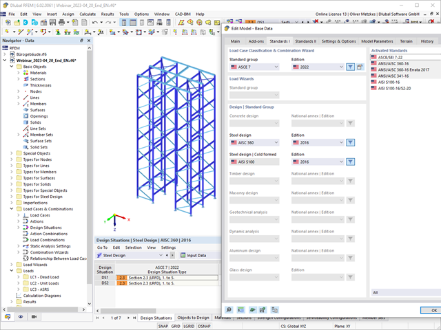
- In addition to Eurocode 3, other international standards are integrated (such as AISC 360, CSA S16, GB 50017, SP 16.13330)
- Consideration of hot-dip galvanizing (DASt guideline 027) in the fire protection design according to EN 1993‑1‑2
- Input option for transverse stiffeners that can be taken into account in the shear buckling analysis
- Lateral-torsional buckling can also be checked for hollow sections (for example, relevant for slender, high rectangular hollow sections)
- Automatic detection of members or member sets valid for the design (for example, automatic deactivation of members with invalid material or members already contained in a member set)
- Design settings can be adjusted individually for each member
- Graphical display of the results in the gross section or the effective section
- Output of the used design check formulas (including a reference to the used equation from the standard)
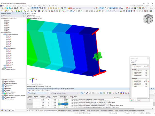
The Torsional Warping (7 DOF) add-on provides you with numerous new possibilities. For example, you can perform the calculation of member structures in RFEM and RSTAB, taking into account the cross-section warping. You can consider the resulting internal forces (N, Vu, Vv, Mt,pri, Mt,sec, Mu, Mv, Mω) in the equivalent stress analysis of the steel design. Please note: This feature is currently not available for the design standards AISC 360‑16 and GB 50017.

The Concrete Design add-on allows you to perform the seismic design of reinforced concrete members according to EC 8. This includes, among other things, the following functionalities:
- Seismic design configurations
- Differentiation of the ductility classes DCL, DCM, DCH
- Option to transfer the behavior factor from a dynamic analysis
- Check of the limit value for the behavior factor
- Capacity design checks of "Strong column - weak beam"
- Detailing and particular rules for curvature ductility factor
- Detailing and particular rules for local ductility

You can select several methods that are available for the eigenvalue analysis:
- Direct Methods
- The direct methods (Lanczos [RFEM], roots of characteristic polynomial [RFEM], subspace iteration method [RFEM/RSTAB], and shifted inverse iteration [RSTAB]) are suitable for small to medium-sized models. You should only use these fast solver methods if your computer has a larger amount of memory (RAM).
- ICG Iteration Method (Incomplete Conjugate Gradient [RFEM])
- In contrast, this method only requires a small amount of memory. Eigenvalues are determined one after the other. It can be used to calculate large structural systems with few eigenvalues.
Use the Structure Stability add-on to perform a nonlinear stability analysis using the incremental method. This analysis delivers close-to-reality results also for nonlinear structures. The critical load factor is determined by gradually increasing the loads of the underlying load case until the instability is reached. The load increment takes into account nonlinearities such as failing members, supports and foundations, and material nonlinearities. After increasing the load, you can optionally perform a linear stability analysis on the last stable state in order to determine the stability mode.
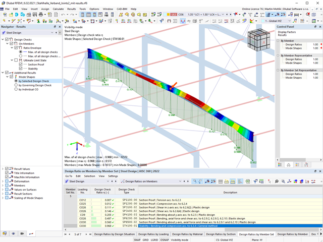
Did you use the eigenvalue solver of the add-on to determine the critical load factor for the stability analysis? Verz well, you can then display the governing mode shape of the object to be designed as a result. The eigenvalue solver is available for the lateral-torsional buckling analysis, depending on the design standard used. You can also use the internal eigenvalue solver for the general method according to EN 1993‑1‑1, 6.3.4.

The soil solids that you want to analyze are summarized in soil massifs.
Use the soil samples as a basis for a definition of the respective soil massif. This way, the program allows for user-friendly generation of the massif, including the automatic determination of the layer interfaces from the sample data, as well as the groundwater level and the boundary surface supports.
Soil massifs provide you with the option to specify a target FE mesh size independently of the global setting for the rest of the structure. You can thus consider the various requirements of the building and soil in the entire model.

Your data are always documented in a multilingual printout report. You can adjust the content at any time and save it as a template. You can also add graphics, texts, MathML formulas, and PDF documents to your report with just a few clicks.
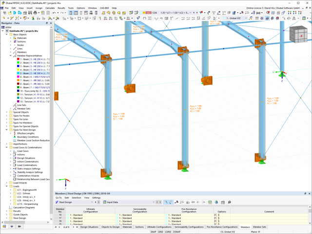
Do you want to perform a stability analysis in the Steel Design add-on? Then it is absolutely necessary to define the effective lengths. To do this, define the nodal supports and effective length factors in the input dialog box. For easy documentation and a comprehensible check of the entries, you can also graphically display the nodal supports and the resulting segments with the corresponding effective length factor in the work window of RFEM/RSTAB.
You can find the serviceability limit state design checks in the result tables of the Steel Design add-on. You can display the design results with all the details at each location of the designed members. Furthermore, graphics are available for you with the result diagrams of the design ratios. This gives you a good overview.
You can also integrate all result tables and graphics into the global printout report of RFEM/RSTAB as a part of the steel design results. Thus, you can display and document the deformations of the entire structure as a part of the RFEM/RSTAB functionality independent of the add-on.

Compared to the RF‑/STABILITY (RFEM 5) and RSBUCK (RSTAB 8) add-on modules, the following new features have been added to the Structure Stability add-on for RFEM 6 / RSTAB 9:
- Activation as a property of a load case or a load combination
- Automated activation of the stability calculation via combination wizards for several load situations in one step
- Incremental load increase with user-defined termination criteria
- Modification of the mode shape normalization without recalculation
- Result tables with filter option