
As you've already learned, the results of a Modal Analysis load case are displayed in the program after a successful calculation. You can thus immediately see the first mode shape graphically or as an animation. You can also easily adjust the representation of the mode shape standardization. Do that directly in the Results navigator, where you have one of four options for the visualization of the mode shapes available for the selection:
- Scaling the value of the mode shape vector uj to 1 (considers the translation components only)
- Selecting the maximum translational component of the eigenvector and setting it to 1
- Considering the entire eigenvector (including the rotation components), selecting the maximum, and setting it to 1
- Setting the modal mass mi for each mode shape to 1 kg
You can find a detailed explanation of the mode shape standardization in the OnlineManual here.

Is the calculation finished? The results of the modal analysis are then available both graphically and in tables. Display the result tables for the load case or the load cases of the modal analysis. Thus, you can see the eigenvalues, angular frequencies, natural frequencies, and natural periods of the structure at first glance. The effective modal masses, modal mass factors, and participation factors are also clearly displayed.

Is your goal to determine the number of mode shapes? The program offers you two methods for this. On the one hand, you can manually define the number of the smallest mode shapes to be calculated. In this case, the number of available mode shapes depends on the degrees of freedom (that is, the number of free mass points multiplied by the number of directions in which the masses act). However, it is limited to 9999. On the other hand, you can set the maximum natural frequency the way that the program determined the mode shapes automatically until reaching the natural frequency set.
.png?mw=640&hash=403c565ab80c4dd45c2d1356634fb74a90428b70)
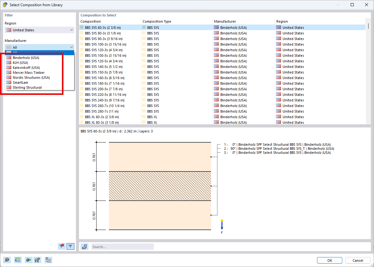
Among others, the following cross-laminated timber manufacturers are available in the layer structure library:
- Binderholz (USA)
- KLH (USA, CAN)
- Kalesnikoff (USA, CAN)
- Nordic Structures (USA, CAN)
- Mercer Mass Timber
- SmartLam
- Sterling Structural
- Superstructures listed in Lignatec Edition 32 "Cross-Laminated Timber of Swiss Production"
By importing a structure from the layer structure library, all relevant parameters are adopted automatically. The library is continually updated.

The Concrete Design add-on allows you to perform the seismic design of reinforced concrete members according to EC 8. This includes, among other things, the following functionalities:
- Seismic design configurations
- Differentiation of the ductility classes DCL, DCM, DCH
- Option to transfer the behavior factor from a dynamic analysis
- Check of the limit value for the behavior factor
- Capacity design checks of "Strong column - weak beam"
- Detailing and particular rules for curvature ductility factor
- Detailing and particular rules for local ductility

You can select several methods that are available for the eigenvalue analysis:
- Direct Methods
- The direct methods (Lanczos [RFEM], roots of characteristic polynomial [RFEM], subspace iteration method [RFEM/RSTAB], and shifted inverse iteration [RSTAB]) are suitable for small to medium-sized models. You should only use these fast solver methods if your computer has a larger amount of memory (RAM).
- ICG Iteration Method (Incomplete Conjugate Gradient [RFEM])
- In contrast, this method only requires a small amount of memory. Eigenvalues are determined one after the other. It can be used to calculate large structural systems with few eigenvalues.
Use the Structure Stability add-on to perform a nonlinear stability analysis using the incremental method. This analysis delivers close-to-reality results also for nonlinear structures. The critical load factor is determined by gradually increasing the loads of the underlying load case until the instability is reached. The load increment takes into account nonlinearities such as failing members, supports and foundations, and material nonlinearities. After increasing the load, you can optionally perform a linear stability analysis on the last stable state in order to determine the stability mode.
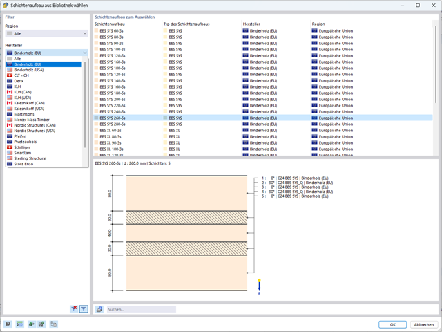
A library for cross-laminated timber panels is implemented in RFEM, from which you can import the manufacturer's layer structures (for example, Binderholz, KLH, Piveteaubois, Södra, Züblin Timber, Schilliger, Stora Enso). In addition to the layer thicknesses and materials, there is also the information about stiffness reductions and the narrow side bonding.
Go to Explanatory Video
Compared to the RF‑/STABILITY (RFEM 5) and RSBUCK (RSTAB 8) add-on modules, the following new features have been added to the Structure Stability add-on for RFEM 6 / RSTAB 9:
- Activation as a property of a load case or a load combination
- Automated activation of the stability calculation via combination wizards for several load situations in one step
- Incremental load increase with user-defined termination criteria
- Modification of the mode shape normalization without recalculation
- Result tables with filter option

Do you know exactly how the form-finding is performed? First, the form-finding process of the load cases with the load case category "Prestress" shifts the initial mesh geometry to an optimally balanced position by means of iterative calculation loops. For this task, the program uses the Updated Reference Strategy (URS) method by Prof. Bletzinger and Prof. Ramm. This technology is characterized by equilibrium shapes that, after the calculation, comply almost exactly with the initially specified form-finding boundary conditions (sag, force, and prestress).
In addition to the pure description of the expected forces or sags on the elements to be formed, the integral approach of the URS also enables a consideration of regular forces. In the overall process, this allows, for example, for a description of the self-weight or a pneumatic pressure by means of corresponding element loads.
All these options give the calculation kernel the potential to calculate anticlastic and synclastic forms that are in an equilibrium of forces for planar or rotationally symmetric geometries. In order to be able to realistically implement both types individually or together in one environment, the calculation provide you with two ways to describe the form-finding force vectors:
- Tension method - description of the form-finding force vectors in space for planar geometries
- Projection method - description of the form-finding force vectors on a projection plane with fixation of the horizontal position for conical geometries

Have you already discovered the tabular and graphical output of masses in mesh points? That's right, this is also part of the modal analysis results in RFEM 6. This way, you can check the imported masses that depend on various settings of the modal analysis. They can be displayed in the Masses in Mesh Points tab of the Results table. The table provides you with an overview of the following results: Mass - Translational Direction (mX, mY, mZ), Mass - Rotational Direction (mφX, mφY, mφZ), and the Sum of Masses. Would it be best for you to have a graphical evaluation as quickly as possible? Then you can also graphically display the masses in mesh points.

As the first results, the program presents you with the critical load factors. You can then perform an evaluation of stability risks. For member models, the resulting effective lengths and critical loads of the members are displayed to you in tables.
Use the next result window to check the normalized eigenvalues sorted by node, member, and surface. The eigenvalue graphic allows you to evaluate the buckling behavior. This makes it easier for you to take countermeasures.
Compared to the RF-FORM-FINDING add-on module (RFEM 5), the following new features have been added to the Form-Finding add-on for RFEM 6:
- Specification of all form-finding load boundary conditions in one load case
- Storage of form-finding results as initial state for further model analysis
- Automatic assignment of the form-finding initial state via combination wizards to all load situations of a design situation
- Additional form-finding geometry boundary conditions for members (unstressed length, maximum vertical sag, low-point vertical sag)
- Additional form-finding load boundary conditions for members (maximum force in member, minimum force in member, horizontal tension component, tension at i-end, tension at j-end, minimum tension at i-end, minimum tension at j-end)
- Material types "Fabric" and "Foil" in material library
- Parallel form-findings in one model
- Simulation of sequentially building form-finding states in connection with the Construction Stages Analysis (CSA) add-on

Once you activate the Form-Finding add-on in the Base Data, a form-finding effect is assigned to the load cases with the load case category "Prestress" in conjunction with the form-finding loads from the member, surface, and solid load catalog. This is a prestress load case. It thus mutates into a form-finding analysis for the entire model with all member, surface, and solid elements defined in it. You reach the form-finding of the relevant member and membrane elements amid the overall model by using special form-finding loads and regular load definitions. These form-finding loads describe the expected state of deformation or force after the form-finding in the elements. The regular loads describe the external loading of the entire system.

The Ponding load type allows you to simulate rain actions on multi-curved surfaces, taking into account the displacements according to the large deformation analysis.
This numerical rainfall process examines the assigned surface geometry and determines which rainfall portions drain away and which rainfall portions accumulate in puddles (water pockets) on the surface. The puddle size then results in a corresponding vertical load for the structural analysis.
For example, you can use this feature in the analysis of approximately horizontal membrane roof geometries subjected to rain loading.
Go to Explanatory VideoIf there is a load case or load combination in the program, the stability calculation is activated. You can define another load case in order to consider initial prestress, for example.
For this, you need to specify whether to perform a linear or nonlinear analysis. Depending on the case of application, you can select a direct calculation method, such as the Lanczos method or the ICG iteration method. Members not integrated in surfaces are usually displayed as member elements with two FE nodes. With such elements, the program cannot determine the local buckling of single members. That's why you have the option to divide members automatically.

Did you know? You can easily define structural modifications in load cases of the Modal Analysis type. This allows you, for example, to individually adjust the stiffnesses of materials, cross-sections, members, surfaces, hinges, and supports. You can also modify stiffnesses for some design add-ons. Once you select the objects, their stiffness properties are adapted to the object type. In this way, you can define them in separate tabs.
Do you want to analyze the failure of an object (for example, a column) in the modal analysis? This is also possible without any problems. Simply switch to the Structure Modification window and deactivate the relevant objects.

The form-finding process gives you a structural model with active forces in the "prestress load case" This load case shows the displacement from the initial input position to the form-found geometry in the deformation results. In the force or stress-based results (member and surface internal forces, solid stresses, gas pressures, and so on), it clarifies the state for maintaining the found form. For the analysis of the shape geometry, the program offers you a two-dimensional contour line plot with the output of the absolute height and an inclination plot for the visualization of the slope situation.
Now, a further calculation and structural analysis of the entire model is performed. For this purpose, the program transfers the form-found geometry including the element-wise strains into a universally applicable initial state. You can now use it in the load cases and load combinations.

The stress and strain results by surface can be output in the surface result table according to the thickness layer.

Compared to the RF‑/DYNAM Pro - Natural Vibrations add-on module (RFEM 5 / RSTAB 8), the following new features have been added to the Modal Analysis add-on for RFEM 6 / RSTAB 9:
- Preset combination coefficients for various standards (EC 8, ASCE, and so on)
- Optional neglect of masses (for example, mass of foundations)
- Methods for determining the number of mode shapes (user-defined, automatic - to reach effective modal mass factors, automatic - to reach the maximum natural frequency)
- Output of modal masses, effective modal masses, modal mass factors, and participation factors
- Masses in mesh points displayed in tables and graphics
- Various scaling options for mode shapes in the Result navigator

When defining the input data for the modal analysis load case, you can consider a load case whose stiffnesses represent the initial position for the modal analysis. How do you do that? As shown in the image, select the "Consider initial state from" option. Now, open the "Initial State Settings" dialog box and define the type Stiffness as the initial state. In this load case, as of which is the initial state taken into account, you can consider the stiffness of the structural system when the tension members fail. The purpose of all of this: The stiffness from this load case is considered in the modal analysis. Thus, you obtain a clearly flexible system.

It is often necessary to neglect masses. This is particularly the case when you want to use the output of the modal analysis for the seismic analysis. For this, 90% of the effective modal mass in each direction is required for the calculation. So you can neglect the mass in all fixed nodal and line supports. The program automatically deactivates the associated masses for you.
You can also manually select the objects whose masses are to be neglected for the modal analysis. We have shown the latter in the image for a better view. A user-defined selection is made the and the objects with their associated mass components are selected to neglect the masses.

You can already see it in the image: Imperfections can also be taken into account when defining a modal analysis load case. The imperfection types that you can use in the modal analysis are notional loads from load case, initial sway via table, static deformation, buckling mode, dynamic mode shape, and group of imperfection cases.

- Calculation of models consisting of member, shell, and solid elements
- Nonlinear stability analysis
- Optional consideration of axial forces from initial prestress
- Four equation solvers for an efficient calculation of various structural models
- Optional consideration of stiffness modifications in RFEM/RSTAB
- Determination of a stability mode greater than the user-defined load increment factor (Shift method)
- Optional determination of the mode shapes of unstable models (to identify the cause of instability)
- Visualization of the stability mode
- Basis for determining imperfection

As soon as the program has completed the calculation, the eigenvalues, natural frequencies and periods are listed. These result windows are integrated in the main program RFEM/RSTAB. You can find all mode shapes of the structure in tables and also have an option to display them graphically and to animate them.
All result tables and graphics are part of the RFEM/RSTAB printout report. In this way, you can ensure clearly arranged documentation. You can also export the tables to MS Excel.

Do you want to consider other loads as masses in addition to the static loads? The program allows that for nodal, member, line and surface loads. For this, you need to select the Mass load type when defining the load of interest. Define a mass or mass components in the X, Y, and Z directions for such loads. For nodal masses, you have an additional option to also specify moments of inertia X, Y, and Z in order to model more complex mass points.

The modal relevance factor (MRF) can help you to assess to which extent specific elements participate in a specific mode shape. The calculation is based on the relative elastic deformation energy of each individual member.
The MRF can be used to distinguish between local and global mode shapes. If multiple individual members show significant MRF (for example, > 20%), the instability of the entire structure or a substructure is very likely. On the other hand, if the sum of all MRFs for an eigenmode is around 100%, a local stability phenomenon (for example, buckling of a single bar) can be expected.
Furthermore, the MRF can be used to determine critical loads and equivalent buckling lengths of certain members (for example, for stability design). Mode shapes for which a specific member has small MRF values (for example, < 20%) can be neglected in this context.
The MRF is displayed by mode shape in the result table under Stability Analysis → Results by Members → Effective Lengths and Critical Loads.

In the modal analysis settings, you have to enter all data that are necessary for the determination of the natural frequencies. These are, for example, mass shapes and eigenvalue solvers.
The Modal Analysis add-on determines the lowest eigenvalues of the structure. Either you adjust the number of eigenvalues or let them determined automatically. Thus, you should reach either effective modal mass factors or maximum natural frequencies. Masses are imported directly from load cases and load combinations. In this case, you have the option to consider the total mass, load components in the global Z-direction, or only the load component in the direction of gravity.
You can manually define additional masses at nodes, lines, members, or surfaces. Furthermore, you can influence the stiffness matrix by importing axial forces or stiffness modifications of a load case or load combination.

- Automatic consideration of masses from self-weight
- Direct import of masses from load cases or load combinations
- Optional definition of additional masses (nodal, linear, or surface masses, as well as inertia masses) directly in the load cases
- Optional neglect of masses (for example, mass of foundations)
- Combination of masses in different load cases and load combinations
- Preset combination coefficients for various standards (EC 8, SIA 261, ASCE 7,...)
- Optional import of initial states (for example, to consider prestress and imperfection)
- Structure Modification
- Consideration of failed supports or members/surfaces/solids
- Definition of several modal analyses (for example, to analyze different masses or stiffness modifications)
- Selection of mass matrix type (diagonal matrix, consistent matrix, unit matrix), including user-defined specification of translational and rotational degrees of freedom
- Methods for determining the number of mode shapes (user-defined, automatic - to reach effective modal mass factors, automatic - to reach the maximum natural frequency - only available in RSTAB)
- Determination of mode shapes and masses in nodes or FE mesh points
- Results of eigenvalue, angular frequency, natural frequency, and period
- Output of modal masses, effective modal masses, modal mass factors, and participation factors
- Masses in mesh points displayed in tables and graphics
- Visualization and animation of mode shapes
- Various scaling options for mode shapes
- Documentation of numerical and graphical results in printout report

In RFEM, you can use these three powerful eigenvalue solvers:
- Root of Characteristic Polynomial
- Method by Lanczos
- Subspace Iteration
RSTAB, on the other hand, provides you with these two eigenvalue solvers:
- Subspace Iteration
- Shifted inverse power method
The selection of the eigenvalue solver depends primarily on your model size.

For a response spectrum analysis of building models, you can display the sensitivity coefficients for the horizontal directions by story.
These key figures allow you to interpret the sensitivity to stability effects.