- The proposed connection can be applied to all selected nodes in the structure
- The location of the connection can be defined using the 'Main' tab of the Add-on dialog box
- The design is performed for all connections in the structure and after the calculation, the results on all connections can be displayed
- The table shows the results for the individual connections, each connection is designed and can be saved separately
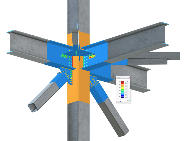
Complex Connection of Horizontal Beams to Column and Connection of Reinforcing Diagonals
The connection model was modeled using about 50 components. The model was created according to the real example of use in structure.
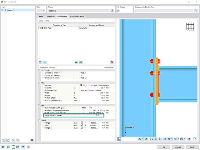
To determine the shear resistance of bolts, you can use the Steel Joints add-on to specify whether there is a shaft or a thread in the shear plane.
Go to Explanatory Video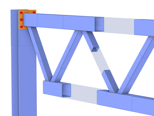
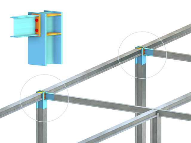
In the case of rectangular cross-sections, you can usually achieve a direct connection by using welds. However, you can also connect them to other cross-sections in the same way. Furthermore, other components such as end plates help you to connect the rectangular cross-sections to other structural components.
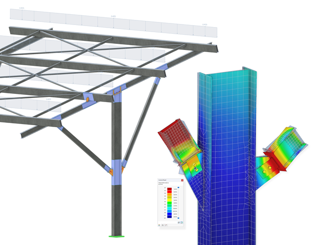
Steel bolted connections with gusset plates on the canopy structure.
Download the structural analysis model and open it with the finite element program RFEM 6 using Steel Joints Add-on.
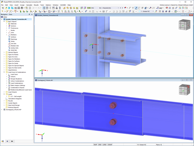
In the Steel Joint add-on, you can design the connections of members with composite cross-sections. Furthermore, you can perform joint design checks for almost all thin-walled cross-sections in the RFEM library.
Go to Explanatory Video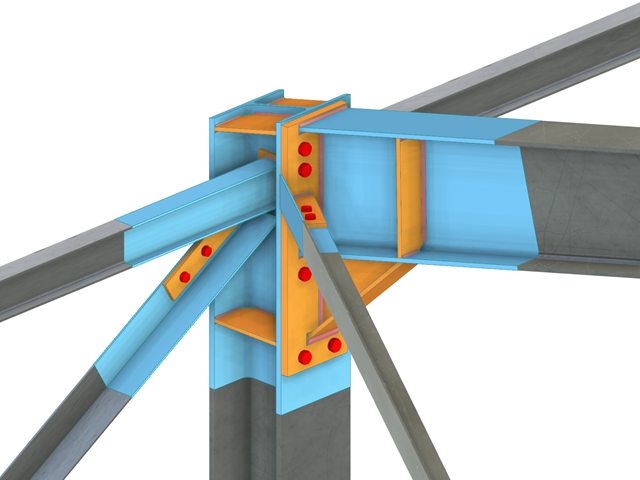
Design of a frame connection with taper and stiffened members. A stress analysis and a buckling stability analysis were carried out for the connection. To display the buckling results, the connection was converted into a separate model.
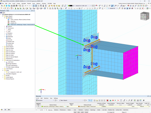
Here, the weld design becomes child's play. Using the specially developed material model "Orthotropic | Plastic | Weld (Surfaces)", you can calculate all stress components plastically. The stress τperpendicular is also considered plastically.
Using this material model you can design welds closer to reality and more efficiently.
Explanatory VideoThe program supports you: It determines the bolt forces on the basis of the FE analysis model and evaluates them automatically. The add-on performs the standard-compliant design of bolt resistance for failure cases, such as tension, shear, hole bearing, and punching, and clearly displays all required coefficients.
Do you want to perform weld design? The welds are modeled as elastic-plastic surface elements, and their stresses are read out from the FE analysis model. The plasticity criteria is set in the way that they represent failure according to AISC J2-4, J2-5 (strength of welds), and J2-2 (strength of base metal). The design can be performed with the partial safety factors of the selected National Annex of EN 1993‑1‑8.
The plates in the connection are designed plastically by comparing the existing plastic strain to the allowable plastic strain. The default setting is 5% according to EN 1993‑1‑5, Annex C, but can be adjusted by user-defined specifications, as well as 5% for AISC 360.
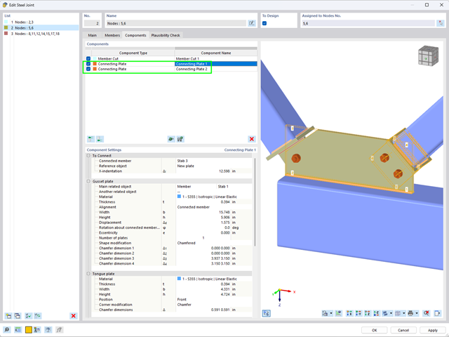
Using the "Connecting Plate" component, you can additionally and automatically create a new gusset plate in the Steel Joints add-on. This saves you separate components, and the other elements, such as a cap plate and a slide plate, are thus automatically taken into account with their dimensions.
Go to Explanatory Video
- Many predefined components: Allow easy input of typical connection situations, such as end plates, angles, multi-wall sheets, cleats, fin plates
- Universally applicable basic components (plates, welds, bolts, auxiliary planes) for entering complex connection situations
- Graphical display of the connection geometry that is updated in parallel with the input
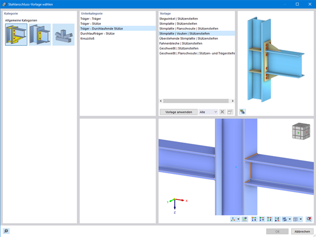
- The Steel Joints Template included in the add-on allows you to select from several connection types and, and once selected, it will be applied to your model.
- Wide range of cross-section shapes: Includes I-sections, channel sections, angles, T-sections, built-up cross-sections, RHS (rectangular hollow sections), and thin-walled sections
- The Template covers connections from three general categories: Rigid, Pinned, Truss
- Automatic adaptation of the connection geometry, even if the structural components are subsequently edited, based on the relative relation of the components

As you've already learned, the results of a Modal Analysis load case are displayed in the program after a successful calculation. You can thus immediately see the first mode shape graphically or as an animation. You can also easily adjust the representation of the mode shape standardization. Do that directly in the Results navigator, where you have one of four options for the visualization of the mode shapes available for the selection:
- Scaling the value of the mode shape vector uj to 1 (considers the translation components only)
- Selecting the maximum translational component of the eigenvector and setting it to 1
- Considering the entire eigenvector (including the rotation components), selecting the maximum, and setting it to 1
- Setting the modal mass mi for each mode shape to 1 kg
You can find a detailed explanation of the mode shape standardization in the OnlineManual here.

RFEM allows you to use a special line hinge to model the special properties of the connection between the reinforced concrete slab and masonry wall. This limits the transferable forces of the connection depending on the specified geometry. You guess right: This means that the material cannot be overloaded.
The program develops interaction diagrams that are applied automatically. They represent the various geometric situations and you can use them to determine the correct stiffness.

Is the calculation finished? The results of the modal analysis are then available both graphically and in tables. Display the result tables for the load case or the load cases of the modal analysis. Thus, you can see the eigenvalues, angular frequencies, natural frequencies, and natural periods of the structure at first glance. The effective modal masses, modal mass factors, and participation factors are also clearly displayed.
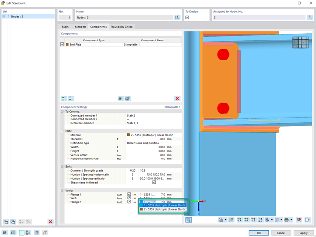
If a weld seam connects two plates with different materials, it is possible to select from a combo box in the Steel Joints add-on which one of both materials should be used for the weld seam.
Go to Explanatory Video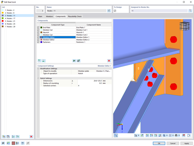
The "Member Editor" component allows you to modify the individual or several member plates in the Steel Joints add-on.
You can use the chamfer, notch, rounding, and hole operations with multiple shapes. It is possible to apply both operations, "Notch" and "Chamfer", for several member plates.
In this way, you can notch flanges from I-sections, for example (see the image).
Go to Explanatory Video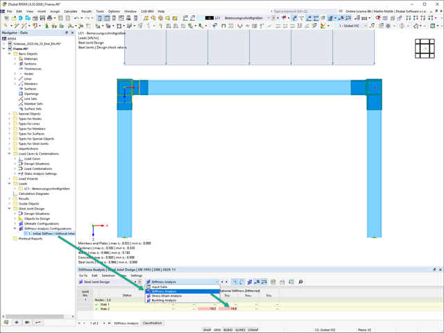
The initial stiffness Sj,ini is a crucial parameter for evaluating whether a connection can be characterized as rigid, semi-rigid, or pinned.
In the "Steel Joints" add-on, you can calculate the initial stiffness Sj,ini according to Eurocode (EN 1993‑1‑8, Section 5.2.2) and AISC (AISC 360-16, Cl. E3.4) with regard to the internal forces N, My, and/or Mz.
The optional automatic transfer of initial stiffnesses allows for a directly transfer as member hinge stiffnesses in RFEM. The entire structure is then recalculated and the resulting internal forces are automatically adopted as loads in the analysis and design of the connection models.
This automated iteration process eliminates the need for manual export and import of data, reducing the amount of work and minimizing potential sources of error.
Explanatory Video: Calculation of Initial Stiffness Sj,ini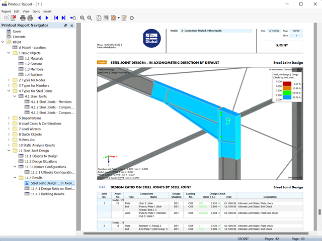
- The results of the connection design can be entered in the printout report
- When creating a new printout report, select the items added from the Steel Joints Add-on
- Use the tool 'Print Graphics to Printout Report' to insert graphics with the results of the connection, including the control panel, into the report
- Printout report contains the specifications of the connection components, design parameters, results and graphics
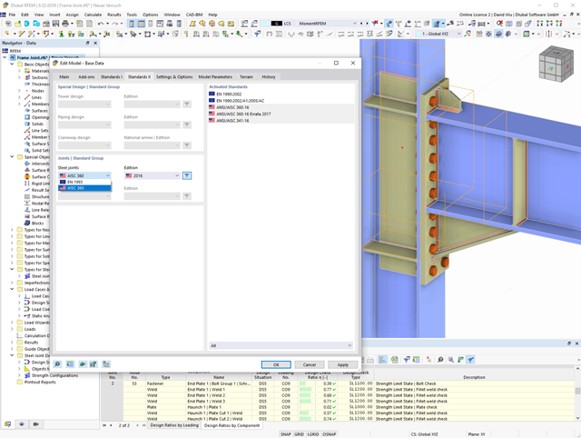
In the Steel Joints add-on, you can design connections according to the American standard ANSI/AISC 360‑16. The following design procedures are integrated:
- Load and Resistance Factor Design (LRFD)
- Allowable Stress Design (ASD)

Is your goal to determine the number of mode shapes? The program offers you two methods for this. On the one hand, you can manually define the number of the smallest mode shapes to be calculated. In this case, the number of available mode shapes depends on the degrees of freedom (that is, the number of free mass points multiplied by the number of directions in which the masses act). However, it is limited to 9999. On the other hand, you can set the maximum natural frequency the way that the program determined the mode shapes automatically until reaching the natural frequency set.

Are you ready for the evaluation? Use the calculation diagrams, which show the distribution of a specific result during the calculation.
You can freely define the layout of the vertical and horizontal axes of the calculation diagram. This allows you, for example, to consider the settlement distribution of a certain node, depending on the load.
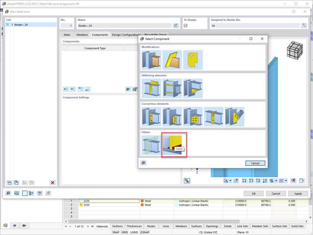
In addition to other predefined components in the design add-on for steel connections, the universal base component "General Weld" can be used to enter complex connection situations.

Do you want to model and analyze the behavior of a soil solid? To ensure this, special suitable material models have been implemented in RFEM.
You can use the modified Mohr-Coulomb model with a linear-elastic ideal-plastic model or a nonlinear elastic model with an oedometric stress-strain relation. The limit criterion, which describes the transition from the elastic area to that of the plastic flow, is defined according to Mohr-Coulomb.
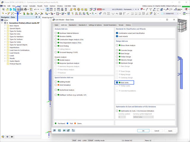
To design a Steel connection, you must have the Steel Joints Add-on enabled. The Add-ons in RFEM 6 are activated in the Add-ons tab of the Edit Model - Base Data window. If the Add-on is active, it is displayed in the navigator.
.png?mw=640&hash=25998fe3470f8e1c154828f202ad6a728b30f00a)
Did you know that To calculate masonry structures, a nonlinear material model has been implemented in RFEM. It is based on the approach of Lourenco, a composite yield surface according to Rankine and Hill. This model allows you to describe and model the structural behavior of masonry and the different failure mechanisms.
The limit parameters were selected in such a way that the design curves used correspond to a normative design curve.
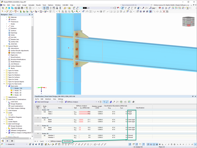
In the Steel Joints add-on, you can classify the joint stiffness.
In addition to the initial stiffness, the table also shows the limit values for hinged and rigid connections for the selected internal forces N, My, and/or Mz. The resulting classification is then displayed in tables as "hinged", "semi-rigid", or "rigid".
Go to Explanatory Video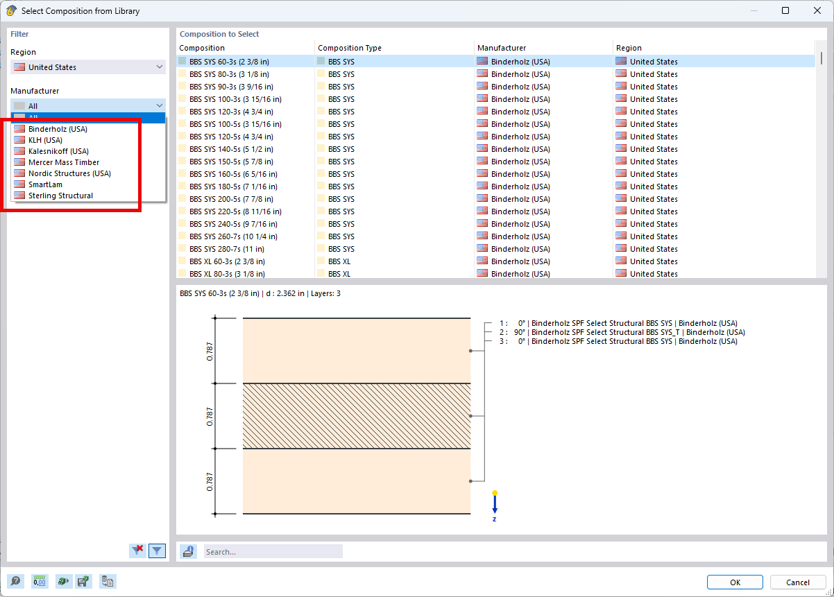.png?mw=640&hash=403c565ab80c4dd45c2d1356634fb74a90428b70)
Among others, the following cross-laminated timber manufacturers are available in the layer structure library:
- Binderholz (USA)
- KLH (USA, CAN)
- Kalesnikoff (USA, CAN)
- Nordic Structures (USA, CAN)
- Mercer Mass Timber
- SmartLam
- Sterling Structural
- Superstructures listed in Lignatec Edition 32 "Cross-Laminated Timber of Swiss Production"
By importing a structure from the layer structure library, all relevant parameters are adopted automatically. The library is continually updated.

Compared to the RF‑SOILIN add-on module (RFEM‑5), the following new features have been added to the Geotechnical Analysis add-on for RFEM 6:
- Creation of the layered soil as a 3D model from the entirety of the defined soil samples
- Recognized material law according to Mohr-Coulomb for soil simulation
- Graphical and tabular output of stresses and strains at any depth of the soil
- Optimal consideration of the soil-structure interaction on the basis of an overall model
For joint components, you can check whether the stability failure is relevant. This requires the Structure Stability add-on for RFEM 6.
In this case, you calculate the critical load factor for all analyzed load combinations and the selected number of mode shapes for the connection model. Compare the smallest critical load factor with the limit value 15 from the standard EN 1993‑1‑1, Clause 5. Furthermore, you can make user-defined adjustment of the limit value. As a result of the stability analysis, the program displays the corresponding mode shapes graphically.
For the stability analysis, RFEM uses the adapted surface model to specifically recognize the local buckling shapes. You can also save and use the model of the stability analysis, including the results, as a separate model file.

The Concrete Design add-on allows you to perform the seismic design of reinforced concrete members according to EC 8. This includes, among other things, the following functionalities:
- Seismic design configurations
- Differentiation of the ductility classes DCL, DCM, DCH
- Option to transfer the behavior factor from a dynamic analysis
- Check of the limit value for the behavior factor
- Capacity design checks of "Strong column - weak beam"
- Detailing and particular rules for curvature ductility factor
- Detailing and particular rules for local ductility