
The parameters of the National Annexes (NA) to Eurocode 3 of the following countries are integrated:
-
 DIN EN 1993-1-1/NA:2016-04 (Germany)
 -
 ÖNORM EN 1993-1-1/NA:2015-12 (Austria)
 -
 SN EN 1993-1-1/NA:2016-07 (Switzerland)
 -
 BDS EN 1993-1-1/NA:2015-10 (Bulgaria)
 -
 BS EN 1993-1-1/NA:2016-07 (United Kingdom)
 -
 CEN EN 1993-1-1/2015-06 (European Union)
 -
 CYS EN 1993-1-1/NA:2015-07 (Cyprus)
 -
 CSN EN 1993-1-1/NA:2016-06 (Czech Republic)
 -
 DS EN 1993-1-1/NA:2015-07 (Denmark)
 -
 ELOT EN 1993-1-1/NA:2017-01 (Greece)
 -
 EVS EN 1993-1-1/NA:2015-08 (Estonia)
 -
 HRN EN 1993-1-1/NA:2016-03 (Croatia)
 -
 I S. EN 1993-1-1/NA:2016-03 (Ireland)
 -
 ILNAS EN 1993-1-1/NA:2015-06 (Luxembourg)
 -
 IST EN 1993-1-1/NA:2015-11 (Iceland)
 -
 LST EN 1993-1-1/NA:2017-01 (Lithuania)
 -
 LVS EN 1993-1-1/NA:2015-10 (Latvia)
 -
 MS EN 1993-1-1/NA:2010-01 (Malaysia)
 -
 MSZ EN 1993-1-1/NA:2015-11 (Hungary)
 -
 NBN EN 1993-1-1/NA:2015-07 (Belgium)
 -
 NEN EN 1993-1-1/NA:2016-12 (Netherlands)
 -
 NF EN 1993-1-1/NA:2016-02 (France)
 -
 NP EN 1993-1-1/NA:2009-03 (Portugal)
 -
 NS EN 1993-1-1/NA:2015-09 (Norway)
 -
 PN EN 1993-1-1/NA:2015-08 (Poland)
 -
 SFS EN 1993-1-1/NA:2015-08 (Finland)
 -
 SIST EN 1993-1-1/NA:2016-09 (Slovenia)
 -
 SR EN 1993-1-1/NA:2016-04 (Romania)
 -
 SS EN 1993-1-1/NA:2019-05 (Singapore)
 -
 SS EN 1993-1-1/NA:2015-06 (Sweden)
 -
 STN EN 1993-1-1/NA:2015-10 (Slovakia)
 -
 TKP EN 1993-1-1/NA:2015-04 (Belarus)
 -
 UNE EN 1993-1-1/NA:2016-02 (Spain)
 -
 UNI EN 1993-1-1/NA:2015-08 (Italy)

- Realistic representation of interaction between a building and soil
- Realistic representation of the influences of the foundation components on each other
- Extensible library of soil properties
- Consideration of several soil samples (probes) at different locations, even outside the building
- Determination of settlements and stress diagrams as well as their graphical and tabular display

Entering soil layers for soil samples is performed in a clearly arranged dialog box. A corresponding graphical representation supports clarity and makes checking the input user-friendly.
An extensible database facilitates the selection of soil material properties. The Mohr-Coulomb model as well as a nonlinear model with stress and strain dependent stiffness are available for a realistic modeling of the soil material behavior.
You can define any number of soil samples and layers. The soil is generated from all entered samples using 3D solids. Assignment to the structure is carried out using coordinates.
The soil body is calculated according to the nonlinear iterative method. The calculated stresses and settlements are displayed graphically and in tables.

The Dlubal structural analysis software does a lot of work for you. The input parameters, which are relevant for the selected standards, are suggested by the program in accordance with the rules. Furthermore, you can enter response spectra manually.
Load cases of the type Response Spectrum Analysis define the direction in which response spectra act and which eigenvalues of the structure are relevant for the analysis. In the spectral analysis settings, you can define details for the combination rules, damping (if applicable), and zero-period acceleration (ZPA).

Did you know that Equivalent static loads are generated separately for each relevant eigenvalue and excitation direction. These loads are saved in a load case of the Response Spectrum Analysis type and RFEM/RSTAB performs a linear static analysis.

The load cases of the type Response Spectrum Analysis contain the generated equivalent loads. First, the modal contributions have to be superimposed with the SRSS or CQC rule. In this case, you can use the signed results based on the dominant mode shape.
Afterwards, the directional components of earthquake actions are combined with the SRSS or the 100% / 30% rule.
_(1).png?mw=640&hash=415f7bbaf70e41679bb0106e1cf91eaa8c493ec9)
- Automatic generation of FE analysis models: The add-on automatically creates a finite element model (FE) of the steel connection in the background.
- Consideration of all internal forces: The calculation and design checks include all internal forces (N, Vy, Vz, My, Mz, MT) and are not limited to planar loading.
- Automatic load transfer: All load combinations are automatically transferred to the FE analysis model of the connection. The loads are transferred directly from RFEM, so manual data input is not necessary.
- Efficient modeling: The add-on saves you time when modeling complex connection situations. You can also save the created FE analysis model and use it further for your own detailed analyses.
- Extensible library: An extensive and extensible library with predefined steel connection templates is available.
- Wide applicability: The add-on is suitable for connections of any type and shape, compatible with almost all rolled, welded, built-up, and thin-walled cross-sections.

- Selection of nodes in the RFEM model, automatic recognition and assignment of the members connected to the node
- Many predefined components available for easy input of typical connection situations (for example, end plates, cleats, fin plates)
- Universally applicable basic components (plates, welds, auxiliary planes) for entering complex connection situations
- No manual editing of the FE model required by the user, the essential calculation settings can be changed via the configuration settings
- Automatic adaptation of the connection geometry, even if the members are subsequently edited, due to the relative relation of the components to each other
- Parallel to the input, a plausibility check is carried out by the program to quickly detect missing input or collisions, for example
- Graphical display of the connection geometry that is updated in parallel with the input
The program supports you: It determines the bolt forces on the basis of the FE analysis model and evaluates them automatically. The add-on performs the standard-compliant design of bolt resistance for failure cases, such as tension, shear, hole bearing, and punching, and clearly displays all required coefficients.
Do you want to perform weld design? The welds are modeled as elastic-plastic surface elements, and their stresses are read out from the FE analysis model. The plasticity criteria is set in the way that they represent failure according to AISC J2-4, J2-5 (strength of welds), and J2-2 (strength of base metal). The design can be performed with the partial safety factors of the selected National Annex of EN 1993‑1‑8.
The plates in the connection are designed plastically by comparing the existing plastic strain to the allowable plastic strain. The default setting is 5% according to EN 1993‑1‑5, Annex C, but can be adjusted by user-defined specifications, as well as 5% for AISC 360.
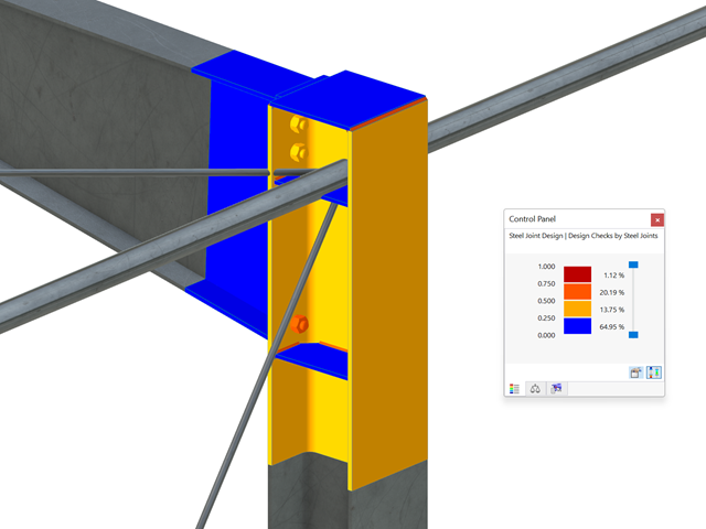
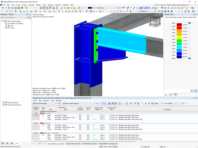
You can display all essential results on the FE model. In this case, you can filter the results separately according to the respective components.
Furthemore, RFEM delivers you all design checks in a tabular form, including the display of the formulas used. If you wish, you can transfer the result tables to the RFEM printout report.
Compared to the RF-/DYNAM Pro - Equivalent Loads add-on module (RFEM 5 / RSTAB 8), the following new features have been added to the Response Spectrum Analysis add-on for RFEM 6 / RSTAB 9:
- Response spectra of numerous standards (EN 1998, DIN 4149, IBC 2018, and so on)
- User-defined response spectra or those generated from accelerograms
- Direction-relative response spectrum approach
- Results are stored centrally in a load case with underlying levels to ensure clarity
- Accidental torsional actions can be taken into account automatically
- Automatic combinations of seismic loads with the other load cases for use in an accidental design situation
Compared to the RF‑SOILIN add-on module (RFEM‑5), the following new features have been added to the Geotechnical Analysis add-on for RFEM 6:
- Creation of the layered soil as a 3D model from the entirety of the defined soil samples
- Recognized material law according to Mohr-Coulomb for soil simulation
- Graphical and tabular output of stresses and strains at any depth of the soil
- Optimal consideration of the soil-structure interaction on the basis of an overall model
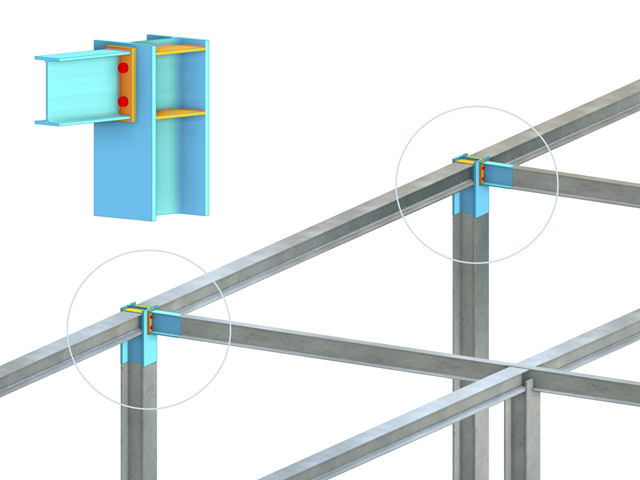
Do you work with steel connections? The Steel Joints add-on for RFEM supports you when analyzing steel connections by using an FE model. In this case, the modeling runs fully automatically in the background. Nevertheless, you can control this process via the simple and familiar input of components. You can then use the loads determined on the FE model for your design of the components according to EN 1993‑1‑8 (including National Annexes).
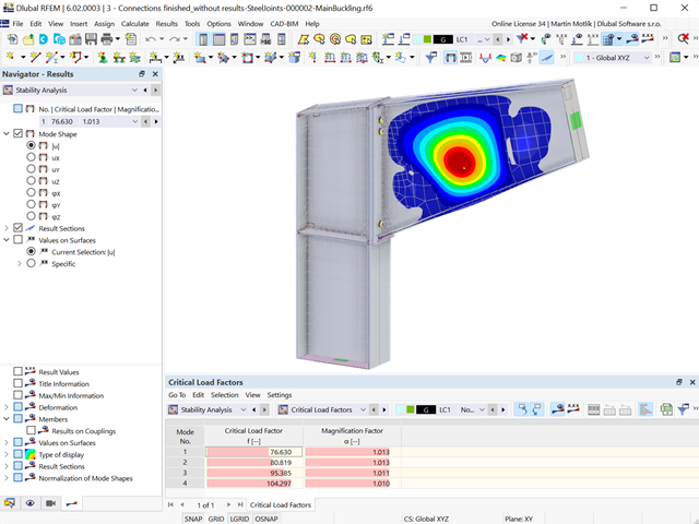
For joint components, you can check whether the stability failure is relevant. This requires the Structure Stability add-on for RFEM 6.
In this case, you calculate the critical load factor for all analyzed load combinations and the selected number of mode shapes for the connection model. Compare the smallest critical load factor with the limit value 15 from the standard EN 1993‑1‑1, Clause 5. Furthermore, you can make user-defined adjustment of the limit value. As a result of the stability analysis, the program displays the corresponding mode shapes graphically.
For the stability analysis, RFEM uses the adapted surface model to specifically recognize the local buckling shapes. You can also save and use the model of the stability analysis, including the results, as a separate model file.
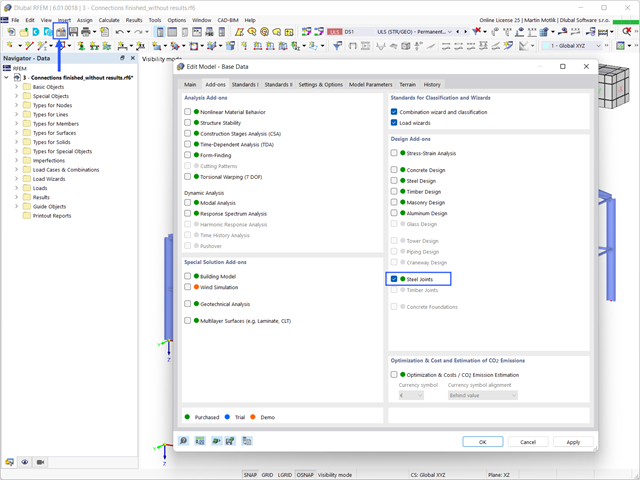
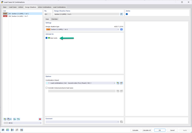
To design a Steel connection, you must have the Steel Joints Add-on enabled. The Add-ons in RFEM 6 are activated in the Add-ons tab of the Edit Model - Base Data window. If the Add-on is active, it is displayed in the navigator.
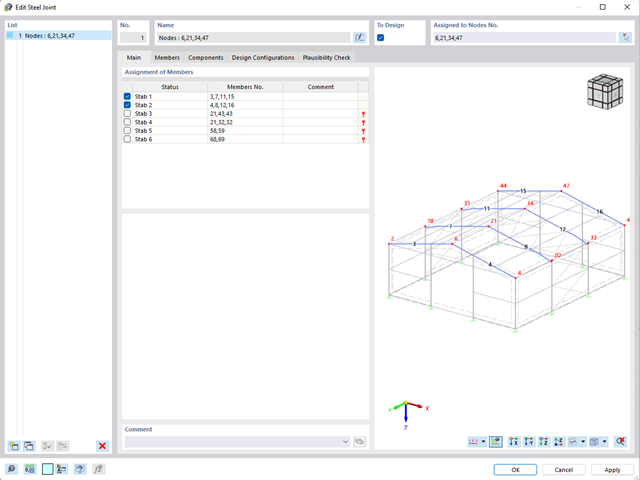
- For a new connection model, you have to select a node in the RFEM model
- After selecting a node, the members connected to the node are automatically recognized and assigned
- In the window for assigning members, select the ones that will be assigned to the connection
- The members marked by us are displayed in the preview window on the right
- Connections can be modeled for multiple nodes in a structure.
- For member settings, select the ones to be supported

- Many predefined components: Allow easy input of typical connection situations, such as end plates, angles, multi-wall sheets, cleats, fin plates
- Universally applicable basic components (plates, welds, bolts, auxiliary planes) for entering complex connection situations
- Graphical display of the connection geometry that is updated in parallel with the input
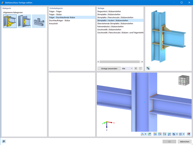
- The Steel Joints Template included in the add-on allows you to select from several connection types and, and once selected, it will be applied to your model.
- Wide range of cross-section shapes: Includes I-sections, channel sections, angles, T-sections, built-up cross-sections, RHS (rectangular hollow sections), and thin-walled sections
- The Template covers connections from three general categories: Rigid, Pinned, Truss
- Automatic adaptation of the connection geometry, even if the structural components are subsequently edited, based on the relative relation of the components
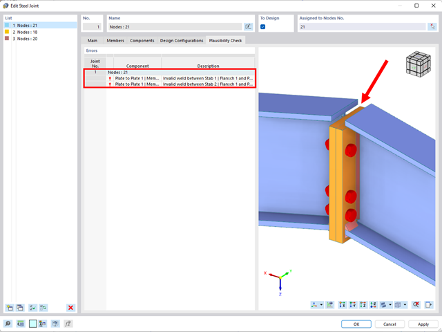
- The program performs a plausibility check in parallel with the input to quickly detect missing entries or collisions.
- If an error occurs, an error message appears describing the problem.
- The steel connections model and the results can be saved as a separate model file
- The resulting stresses and the results of the stability analysis (joint buckling) can be displayed in a separate model
- In the saved model, you can run a deformation animation on the connection
- Connection components are converted to surfaces and members when they are saved
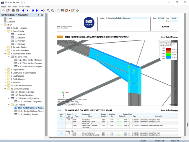
- The results of the connection design can be entered in the printout report
- When creating a new printout report, select the items added from the Steel Joints Add-on
- Use the tool 'Print Graphics to Printout Report' to insert graphics with the results of the connection, including the control panel, into the report
- Printout report contains the specifications of the connection components, design parameters, results and graphics
- The proposed connection can be applied to all selected nodes in the structure
- The location of the connection can be defined using the 'Main' tab of the Add-on dialog box
- The design is performed for all connections in the structure and after the calculation, the results on all connections can be displayed
- The table shows the results for the individual connections, each connection is designed and can be saved separately
- The design of the connection components is performed according to AISC 360 and Eurocode EN 1993‑1‑8.
- After activating the add-on, it is necessary to activate the design situations for Steel Connections in the "Load Cases and Combinations" dialog box.
- The design of the connection stability (buckling) requires the "Structure Stability" add-on.
- You can run the calculation using the table or the icon in the top bar.
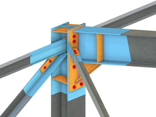
Design of a frame connection with taper and stiffened members. A stress analysis and a buckling stability analysis were carried out for the connection. To display the buckling results, the connection was converted into a separate model.
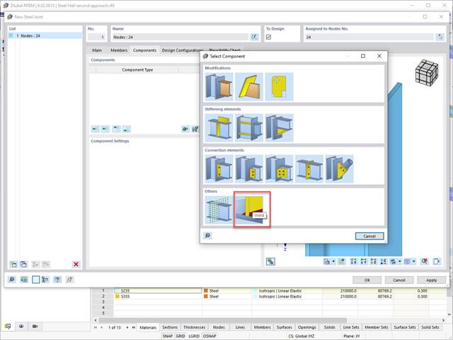
In addition to other predefined components in the design add-on for steel connections, the universal base component "General Weld" can be used to enter complex connection situations.

Do you want to model and analyze the behavior of a soil solid? To ensure this, special suitable material models have been implemented in RFEM.
You can use the modified Mohr-Coulomb model with a linear-elastic ideal-plastic model or a nonlinear elastic model with an oedometric stress-strain relation. The limit criterion, which describes the transition from the elastic area to that of the plastic flow, is defined according to Mohr-Coulomb.

Enter and model a soil solid directly in RFEM. You can combine the soil material models with all common RFEM add-ons.
This allows you to easily analyze the entire models with a complete representation of the soil-structure interaction.
All parameters required for the calculation are automatically determined from the material data that you have entered. The program then generates the stress-strain curves for each FE element.

Did you know? You can enter the soil layers that you have obtained from the subsoil expertises done in the locations into the program in the form of soil samples. Assign the explored soil materials, including their material properties, to the layers.
For the definition of the samples, you can enter the data in tables as well as in the respective editing dialog box. Furthermore, you can also specify the groundwater level in the soil samples.

The soil solids that you want to analyze are summarized in soil massifs.
Use the soil samples as a basis for a definition of the respective soil massif. This way, the program allows for user-friendly generation of the massif, including the automatic determination of the layer interfaces from the sample data, as well as the groundwater level and the boundary surface supports.
Soil massifs provide you with the option to specify a target FE mesh size independently of the global setting for the rest of the structure. You can thus consider the various requirements of the building and soil in the entire model.
.png?mw=640&hash=55038d2a1591f62179796666cb9b2fede0274e19)
A graphical and tabular output of the results for deformations, stresses, and strains helps you when determining the soil solids. To achieve this, use the special filter criteria for targeted selection of results.
The program doesn't leave you alone with the results. If you want to graphically evaluate the results in the soil solids, you can use the guide objects. For example, you can define clipping planes. This allows you to view the corresponding results in any plane of the soil solid.
And not just that. The utilization of result sections and clipping boxes facilitates the precise graphical analysis of the soil solid.
You already know that it is possible to model and analyze a soil and a structure in the entire model. As a result, you have explicitly taken into account the soil-structure interaction. By modifying a component, you achieve the immediate correct consideration in the analysis as well as in the results for the entire system of the soil and structure.