
In RFEM and RSTAB, you can visualize the flow field quantities of pressure, velocity, turbulence kinetic energy, and turbulence dissipation rate for the wind simulation.
The clipping planes are aligned with the respective wind direction.
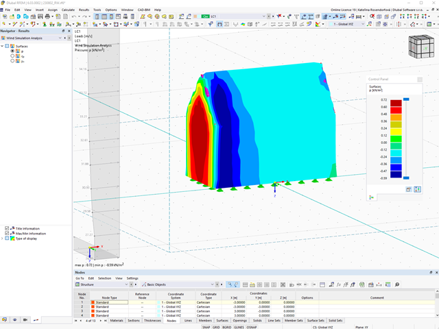
You can display the RWIND results directly in the main program. In the Navigator - Results, select the Wind Simulation Analysis result type from the list above.
Currently, the following results are available, which refer to the RWIND computational mesh:
- Surface pressure
- Surface cp coefficient
- Wall distance y+ (steady flow)
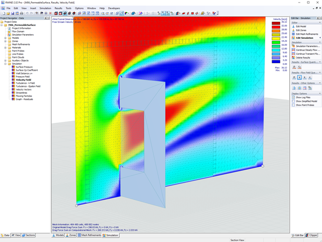
Use RWIND 2 Pro to easily apply a permeability to a surface. All you need is the definition of
- the Darcy coefficient D,
- the inertial coefficient I, and
- the length of the porous medium in the direction of flow L,
to define a pressure boundary condition between the front and back of a porous zone. Due to this setting, you obtain the flow through this zone with a two-part result display on both sides of the zone area.
But that's not all. Furthermore, the generation of a simplified model recognizes permeable zones and takes into account the corresponding openings in the model coating. Can you waive an elaborate geometric modeling of the porous element? Understandable – we have good news for you then! With a pure definition of the permeability parameters, you can avoid complex geometric modeling of the porous element. Use this feature to simulate permeable scaffolding, dust curtains, mesh structures, and so on.
More Information
RFEM 6 and RSTAB 9 support the ergonomically optimized utilization of a mobile 3D mouse by 3Dconnexion.
With a 3D mouse, you can simultaneously move, zoom, and flip a 3D model on the screen beyond the use of a regular mouse. The 3D mouse complements the conventional computer mouse and is operated with your free hand. Therefore, you can streamline the workflow if you operate a 3D mouse with your non-dominant hand, in addition to the normal mouse.

Do you want to model and analyze the behavior of a soil solid? To ensure this, special suitable material models have been implemented in RFEM.
You can use the modified Mohr-Coulomb model with a linear-elastic ideal-plastic model or a nonlinear elastic model with an oedometric stress-strain relation. The limit criterion, which describes the transition from the elastic area to that of the plastic flow, is defined according to Mohr-Coulomb.
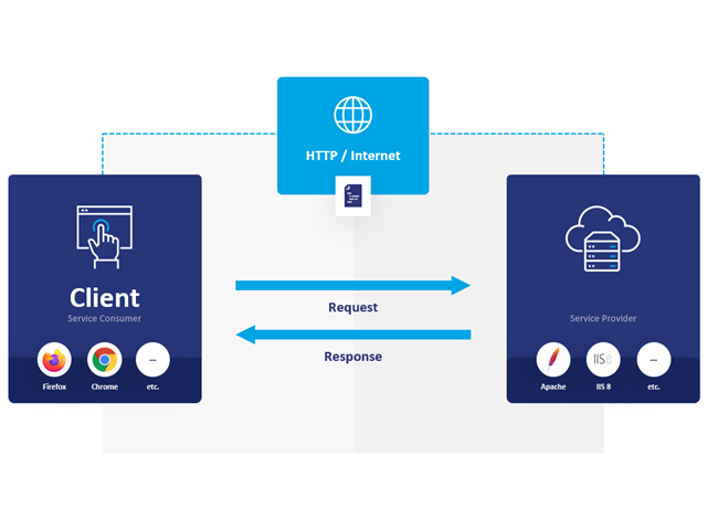
WebService and API provide you various scope of application. We have summarized some ideas as to how WebService and API can support your company:
- Creating additional applications for RFEM 6, RSTAB 9, and RSECTION 1
- Possibility to make the workflows more efficient (for example, model definition and input) and to integrate RFEM 6, RSTAB 9, and RSECTION 1 into your company applications
- Simulating and calculating several design options
- Running optimization algorithms for size, shape, and/or topology
- Accessing the calculation results
- Generation of printout reports in the PDF format
The level of quality of the work is automatically increased not only by the algorithmic model definitions, but also by:
- Extending / consolidating RFEM 6, RSTAB 9, and RSECTION 1 with your own controls
- Increased interoperability between the individual software used to complete a project
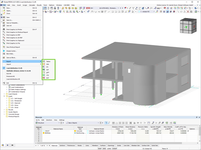
An improvement that will benefit your smooth workflow: You can now export your RFEM and RSTAB models in XML, SAF, and VTK (results from RWIND).
The stand-alone program RWIND 2 takes care of fresh air. It is used for the numerical simulation of wind flow and is available in a Basic as well as a Pro version. What additional features does RWIND Pro offer you? It allows for the calculation of transient incompressible turbulent wind flows (in addition to the stationary ones in RWIND Basic). But that's not all. Intrested to learn more? Find out more here:

- Calculation of stationary incompressible turbulent wind flow using the SimpleFOAM solver from the OpenFOAM® software package
- Numerical scheme according to the first and second order
- Turbulence models RAS k-ω and RAS k-ε
- Consideration of surface roughness depending on model zones
- Model design via VTP, STL, OBJ, and IFC files
- Operation via bidirectional interface of RFEM or RSTAB for importing model geometries with standard-based wind loads and exporting wind load cases with probe-based printout report tables
- Intuitive model changes via drag & drop and graphical adjustment assistance
- Generation of a shrink-wrap mesh envelope around the model geometry
- Consideration of environmental objects (buildings, terrain, and so on)
- Height-dependent description of the wind load (wind speed and turbulence intensity)
- Automatic meshing depending on a selected depth of detail
- Consideration of layer meshes near the model surfaces
- Parallelized calculation with optimal utilization of all processor cores of a computer
- Graphical output of the surface results on the model surfaces (surface pressure, Cp coefficients)
- Graphical output of the flow field and vector results (pressure field, velocity field, turbulence – k-ω field, and turbulence – k-ε field, velocity vectors) on Clipper/Slicer planes
- Display of 3D wind flow via animated streamline graphics
- Definition of point and line probes
- Multilingual user interface (German, English, Czech, Spanish, French, Italian, Polish, Portuguese, Russian, and Chinese)
- Calculations of several models in one batch process
- Generator for creating rotated models to simulate different wind directions
- Optional interruption and continuation of the calculation
- Individual color panel per result graphic
- Display of diagrams with separate output of results on both sides of a surface
- Output of the dimensionless wall distance y+ in the mesh inspector details for the simplified model mesh
- Determination of the shear stress on the model surface from the flow around the model
- Calculation with an alternative convergence criterion (you can select between the residual types pressure or flow resistance in the simulation parameters)
- Calculation of transient incompressible turbulent wind flow with the BlueDyMSolver solver
- LES SpalartAllmarasDDES turbulence model
- Consideration of stationary solution as initial state for transient calculation
- Automatic determination of analysis period and time steps
- Use of intermediate results during the calculation
- Organized display of time-varying results via time step units
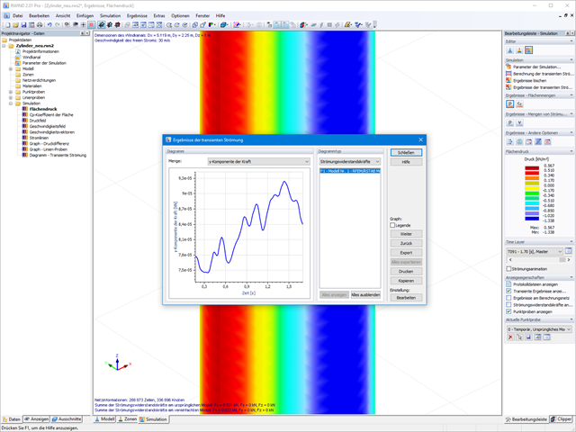
- Diagram of drag force and point probe results over analysis time
- Display of line probe results for any time steps in a diagram
- Freely adjustable wind permeability for surfaces (Go to Product Feature)
RWIND Basic uses a numerical CFD model (Computational Fluid Dynamics) to simulate wind flows around your objects using a digital wind tunnel. The simulation process determines specific wind loads acting on your model surfaces from the flow result around the model.
A 3D volume mesh is responsible for the simulation itself. For this, RWIND Basic performs an automatic meshing on the basis of freely definable control parameters. For the calculation of wind flows, RWIND Basic provides you with a stationary solve and RWIND Pro provides a transient solver for incompressible turbulent flows. Surface pressures resulting from the flow results are extrapolated onto the model for each time step.
By solving the numerical flow problem, you can obtain the following results on and around the model:
- Pressure on structure surface
- Coefficient Cp distribution on the structure surfaces
- Pressure field about the structure geometry
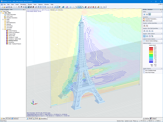
- Velocity field about the structure geometry
- Turbulence k-ω field about the structure geometry
- Turbulence k-ε field about the structure geometry
- Velocity vectors about the structure geometry
- Streamlines about the structure geometry
- Forces on member-shaped structures that were originally generated from member elements
- Convergence diagram
- Direction and size of the flow resistance of the defined structures
Despite this amount of information, RWIND 2 remains clearly arranged, as is typical for the Dlubal programs. You can specify freely definable zones for a graphic evaluation. Voluminously displayed flow results about the structure geometry are often confusing – you know the problem for sure. That's why RWIND Basic provides freely movable section planes for the separate display of the "solid results" in a plane. For the 3D branched streamline result, you have an option to select between a static and an animated display in the form of moving line segments or particles. This option helps you to represent the wind flow as a dynamic effect.
You can export all results as a picture or, especially for the animated results, as a video.
Discover the new features in RFEM and RSTAB for the determination of wind loads using RWIND:
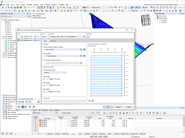
- Useful load wizards for generating wind load cases with different flow fields in different wind directions
- Wind load cases with freely assignable analysis settings including a user-defined specification of the wind tunnel size and wind profile
- Comprehensive display of the wind tunnel with input wind profile and turbulence intensity profile
- Visualization and use of the RWIND simulation results
- Global definition of a terrain (horizontal planes, inclined plane, table)
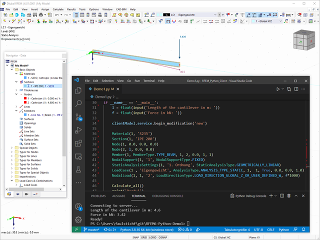
WebService and API allows you to communicate with RFEM, RSTAB, and RSECTION via high-level functions. You can use it to create your web or desktop applications and optimize your workflow. There is also an RFEM 6 server that runs on your computer without a GUI, but only responds to your WebService requests.
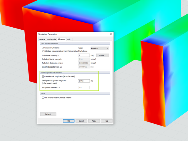
Utilize the RWIND Simulation program to consider a surface roughness of the model surface by applying a modified wall boundary condition. The numerical model is based on the assumption that grains with a certain diameter are arranged homogeneously on the model surface, similar to sandpaper. The grain diameter is described with the parameter Ks and the distribution with the parameter Cs. By considering the wall roughness, the numerical flow simulation can capture reality more closely.
- 3D incompressible wind flow analysis with OpenFOAM® software package
- Direct model import from RFEM or RSTAB including neighboring and terrain models (3DS, IFC, STEP files)
- Model design via STL or VTP files independent of RFEM or RSTAB
- Simple model changes using Drag and Drop and graphical adjustment assistance
- Automatic corrections of the model topology with shrink wrap networks
- Option to add objects from the environment (buildings, terrain ...)
- Wind load determined over the height of the building, depending on standard-specific parameters (velocity, turbulence intensity)
- K-epsilon and K-omega turbulence models
- Automatic mesh generation adjusted to the selected depth of detail
- Parallel calculation with optimal utilization of the capacity of multicore computers
- Results in just minutes for low-resolution simulations (up to 1 million cells)
- Results within a few hours for simulations with medium/high resolution (1‑10 million cells)
- Graphical display of results on the Clipper/Slicer planes (scalar and vector fields)
- Graphical display of streamlines
- Streamline animation (optional video creation)
- Definition of point and line probes
- Display of aerodynamic pressure coefficients
- Graphical display of turbulence properties in the wind field
- Optional meshing using the boundary layer option for the area near the model surface
- Consideration of rough model surfaces possible
- Optional use of a seond-order numerical Order
- Multilingual user interface (for example, German, English, Spanish, French)
- Documentation possible in the RFEM and RSTAB printout report
Work on your models with efficient and precise calculations in the digital wind tunnel. RWIND 2 uses a numerical CFD model (Computational Fluid Dynamics) to simulate wind flows around objects. Specific wind loads are generated from the simulation process for RFEM or RSTAB.
RWIND 2 performs this simulation using a 3D volume mesh. The program provides automatic meshing; you can easily set the entire mesh density as well as the local mesh refinement on the model using a few parameters. A numerical solver for incompressible turbulent flows is used to calculate the wind flows and the surface pressures on the model. The results are then extrapolated to your model. RWIND 2 is designed to work with different numerical solvers.
We currently recommend using the OpenFOAM® software package, which has provided very good results in our tests and is also a frequently used tool for CFD simulations. Alternative numerical solvers are under development.
Always keep an eye on your results. In addition to the resulting load cases in RFEM or RSTAB (see below), the results from the aerodynamics analysis in RWIND 2 represent the flow problem as a whole:
- Pressure on structure surface
- Pressure field about structure geometry
- Velocity field about structure geometry
- Velocity vectors about structure geometry
- Flow lines about structure geometry
- Forces on member-shaped structures that were originally generated from member elements
- Convergence diagram
- Direction and size of the flow resistance of the defined structures
These results are displayed in the RWIND 2 environment and evaluated graphically. The flow results around the structure geometry in the overall display are rather confusing, but the program has a solution for this. In order to present clearly arranged results, freely movable section planes are displayed for the separate display of the 'solid results' in a plane. Accordingly, for the 3D branched streamline result, the program presents you an animated display in the form of moving lines or particles in addition to the static one. This option helps to represent the wind flow as a dynamic effect.
You can export all results as a picture or, especially for the animated results, as a video.
SHAPE-THIN includes an extensive library of rolled and parameterized cross-sections. They can be composed or supplemented by new elements. It is possible to model a section consisting of different materials.
Graphical tools and functions allow for modeling complex section shapes in the usual way common for CAD programs. The graphical entry provides the option of setting point elements, fillet welds, arcs, parameterized rectangular and circular sections, ellipses, elliptical arcs, parabolas, hyperbolas, spline, and NURBS. Alternatively, it is possible to import a DXF file that is used as the basis for further modeling. You can also use guidelines for modeling.
Furthermore, parameterized input allows you to enter model and load data in a specific way so they depend on certain variables.
Elements can be divided or attached to other objects graphically. SHAPE-THIN automatically divides the elements and provides for an uninterrupted shear flow by introducing dummy elements. In the case of dummy elements, you can define a specific thickness to control the shear transfer.
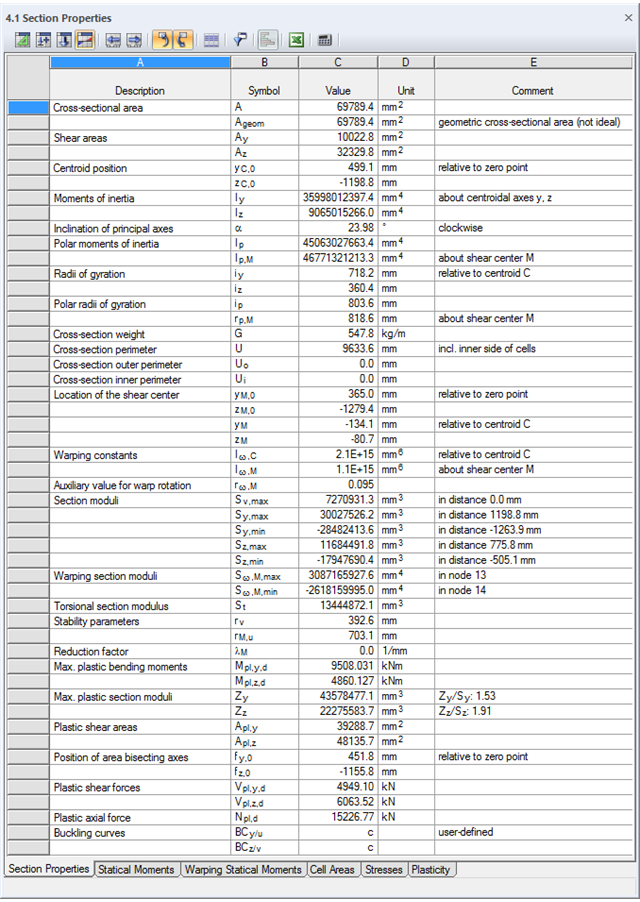
SHAPE-THIN determines the section properties and stresses of any open, closed, built-up, or non-connected cross-sections.
- Section Properties
- Cross-sectional area A
- Shear areas Ay, Az, Au, and Av
- Centroid position yS, zS
- moments of area 2 degrees Iy, Iz, Iyz, Iu, Iv, Ip, Ip,M
- Radii of gyration iy, iz, iyz, iu, iv, ip, ip,M
- Inclination of principal axes α
- Cross-section weight G
- Cross-section perimeter U
- torsional constants of area degrees IT, IT,St.Venant, IT,Bredt, IT,s
- Location of the shear center yM, zM
- Warping constants Iω,S, Iω,M or Iω,D for lateral restraint
- Max/min section moduli Sy, Sz, Su, Sv, Sω,M with locations
- Section ranges ru, rv, rM,u, rM,v
- Reduction factor λM
- Plastic Cross-Section Properties
- Axial force Npl,d
- Shear forces Vpl,y,d, Vpl,z,d, Vpl,u,d, Vpl,v,d
- Bending moments Mpl,y,d, Mpl,z,d, Mpl,u,d, Mpl,v,d
- Section moduli Zy, Zz, Zu, Zv
- Shear areas Apl,y, Apl,z, Apl,u, Apl,v
- Position of area bisecting axes fu, fv,
- Display of the inertia ellipse
- First moments of area Qu, Qv, Qy, Qz with location of maxima and specification of shear flow
- Warping coordinates ωM
- moments of area (warping areas) Sω,M
- Cell areas Am of closed cross-sections
- Normal stresses σx due to axial force, bending moments, and warping bimoment
- Shear stresses τ from shear forces as well as primary and secondary torsional moments
- Equivalent stresses σv with customizable factor for shear stresses
- Stress ratios, related to limit stresses
- Stresses for element edges or center lines
- Weld stresses in fillet welds
- Section properties of non-connected cross-sections (cores of high-rise buildings, composite sections)
- Shear wall shear forces due to bending and torsion
- Plastic capacity design with determination of the enlargement factor αpl
- Check of the c/t-ratios following the design methods el-el, el-pl or pl-pl according to DIN 18800
All results are arranged in result windows sorted by different topics. The design values are illustrated in the corresponding cross-section graphic. The design details cover all intermediate values.
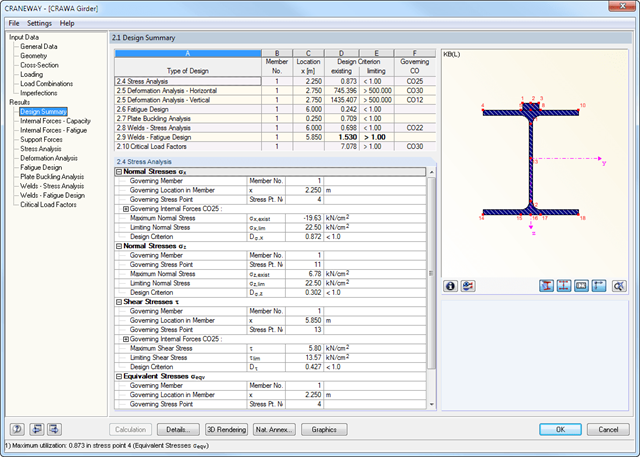
General Stress Analysis
CRANEWAY performs the general stress analysis of a craneway girder by calculating the existing stresses and comparing them with the limit normal, limit shear, and limit equivalent stresses. Welds are also subjected to the general stress analysis with regard to parallel and vertical shear stresses and their superposition.
Fatigue Design
Fatigue design is performed for up to three cranes operating at the same time, based on the nominal stress concept according to EN 1993-1-9. In the case of fatigue design according to DIN 4132, a stress curve of crane passages is recorded for each stress point and evaluated according to the Rainflow method.
Buckling Analysis
Buckling analysis considers the local introduction of wheel loads according to the EN 1993-6 or DIN 18800-3 standards.
Deformation,
Deformation analysis is performed separately for the vertical and horizontal directions. The available related displacements are compared to the allowable values. You can specify the allowable deformation ratios individually in the calculation parameters.
Lateral-torsional buckling analysis
The lateral-torsional buckling analysis is performed in accordance with the second-order analysis for torsional buckling considering imperfections. The general stress analysis has to be fulfilled with the critical load factor greater than 1.00. As a result, CRANEWAY displays the corresponding critical load factor for all load combinations of the stress analysis.
Support forces
The program determines all support forces on the basis of the characteristic loads, including dynamic factors.
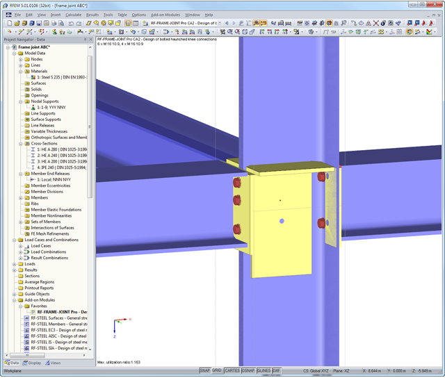
First, the module combines governing designs of the column and the horizontal beam and displays the connection geometry in a result table. The other result tables include all important design details such as flow line lengths, load-bearing capacity of screws, weld stresses, or connection stiffnesses. All connections are visualized in a 3D rendering graphic.
Dimensions, material specifications, and welds that are important for the construction of the connection are visible immediately and can be printed out. It is possible to visualize the connections in RF-/FRAME-JOINT Pro or directly in the RFEM/RSTAB model. All graphics can be included in the RFEM/RSTAB printout report or printed directly. Due to the scaled output, an optimal visual check is possible as early as in the design phase.