113 Wyniki
Wyświetl wyniki:
Sortuj według:

Podczas definiowania etapu budowy i obciążenia można wyświetlić zależności graficznie za pomocą schematu blokowego.

W rozszerzeniu Połączenie stalowe można rozmieszczać obiekty w odniesieniu do innych obiektów.

W rozszerzeniu Połączenia stalowe można używać nie tylko zwykłych typów prętów 'Belka', 'Kratownica' itd., ale także typu pręta 'Belka wynikowa' oraz przekroje z elementów powierzchniowych. Należy wybrać odpowiedni przekrój dla belki wynikowej, a następnie zdefiniować otwory prętowe w modelu powierzchniowym za pomocą edytora prętów.

Komponent 'Kontakt powierzchniowy' w rozszerzeniu Połączenia stalowe umożliwia uwzględnienie kontaktu ciśnieniowego między dwiema równoległymi płytami/płytami prętowymi. W takim przypadku można opcjonalnie uwzględnić tarcie między powierzchniami

Komponent "Stub" jest dostępny w rozszerzeniu Połączenia stalowe. Umożliwia ona wydłużenie pręta za pomocą połączenia płatwi z innym prętem (krótkiem) i połączenie go z komponentem odniesienia.

W rozszerzeniu Połączenia stalowe można teraz układać płyty w różne kształty geometryczne. Oprócz „Prostokąta” i „Okręgu” dostępny jest nowy kształt „Wielokąt”. Forma wielokąta jest określana przez zdefiniowaną współrzędną punktu.

- 002161
- Ogólne informacje
- Optymalizacja i koszty | Szacowanie emisji CO2 RFEM 6
- Optymalizacja i koszty | Szacowanie emisji CO2 RSTAB 9
Obie metody optymalizacji mają jedną wspólną cechę. Na końcu procesu wyświetlają listę wariacji modelu na podstawie przechowywanych danych. Można tu znaleźć szczegóły na temat wyniku decydującego dla optymalizacji i odpowiadające mu wartości parametrów. Lista jest zorganizowana w porządku malejącym. Zakładane najlepsze rozwiązanie znajduje się na górze. W takim przypadku wynik optymalizacji wraz z wyznaczoną wartością jest najbardziej zbliżony do kryterium optymalizacji. Wszystkie dodatkowe wyniki pokazują wykorzystanie < 1. Ponadto, po zakończeniu analizy, program dostosuje wartości na globalnej liście parametrów, aby odpowiadały tym dla optymalnego rozwiązania.
W oknach dialogowych materiałów znajdują się dodatkowe zakładki "Oszacowanie kosztów" i "Oszacowanie emisji CO2". Tutaj wyświetlane są indywidualne szacunkowe sumy przydzielonych prętów, powierzchni i objętości na jednostkę masy, objętości i powierzchni. Dodatkowo zakładki te podają całkowity koszt i emisję wszystkich przydzielonych do konstrukcji materiałów. Zapewnia to dobry przegląd projektu.
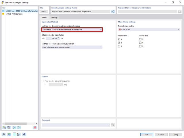
Rozszerzenie Analiza modalna umożliwia automatyczne zwiększanie poszukiwanych wartości własnych do momentu osiągnięcia zdefiniowanego współczynnika efektywnej masy modalnej. Uwzględniane są wszystkie kierunki translacyjne, które zostały aktywowane jako masy do analizy modalnej.
W ten sposób można łatwo obliczyć wymagane 90% efektywnej masy modalnej dla metody spektrum odpowiedzi.

W konfiguracji granicznej dla wymiarowania połączenia stalowego istnieje możliwość modyfikacji granicznego odkształcenia plastycznego dla spoin.
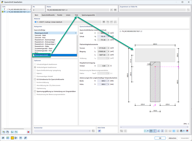
W rozszerzeniu Analiza etapów budowy (CSA) można używać przekrojów złożonych, dzięki zastosowaniu przekrojów etapowanych. Ten typ przekroju umożliwia aktywację lub dezaktywację poszczególnych części przekroju typu "Parametryczny - Masywny II" na poszczególnych etapach budowy.
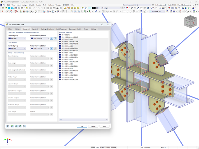
Parametry załączników krajowych (NA) do Eurokodu 3 z następujących krajów są zintegrowane:
-
 DIN EN 1993-1-1/NA:2016-04 (Niemcy)
 -
 ÖNORM EN 1993-1-1/NA:2015-12 (Austria)
 -
 SN EN 1993-1-1/NA:2016-07 (Szwajcaria)
 -
 BDS EN 1993-1-1/NA:2015-10 (Bułgaria)
 -
 BS EN 1993-1-1/NA:2016-07 (Wielka Brytania)
 -
 CEN EN 1993-1-1/2015-06 (Unia Europejska)
 -
 CYS EN 1993-1-1/NA:2015-07 (Cypr)
 -
 CSN EN 1993-1-1/NA:2016-06 (Republika Czeska)
 -
 DS EN 1993-1-1/NA:2015-07 (Dania)
 -
 ELOT EN 1993-1-1/NA:2017-01 (Grecja)
 -
 EVS EN 1993-1-1/NA:2015-08 (Estonia)
 -
 HRN EN 1993-1-1/NA:2016-03 (Chorwacja)
 -
 I S. EN 1993-1-1/NA:2016-03 (Irlandia)
 -
 ILNAS EN 1993-1-1/NA:2015-06 (Luksemburg)
 -
 IST EN 1993-1-1/NA:2015-11 (Islandia)
 -
 LST EN 1993-1-1/NA:2017-01 (Litwa)
 -
 LVS EN 1993-1-1/NA:2015-10 (Łotwa)
 -
 MS EN 1993-1-1/NA:2010-01 (Malezja)
 -
 MSZ EN 1993-1-1/NA:2015-11 (Węgry)
 -
 NBN EN 1993-1-1/NA:2015-07 (Belgia)
 -
 NEN EN 1993-1-1/NA:2016-12 (Holandia)
 -
 NF EN 1993-1-1/NA:2016-02 (Francja)
 -
 NP EN 1993-1-1/NA:2009-03 (Portugalia)
 -
 NS EN 1993-1-1/NA:2015-09 (Norwegia)
 -
 PN EN 1993-1-1/NA:2015-08 (Polska)
 -
 SFS EN 1993-1-1/NA:2015-08 (Finlandia)
 -
 SIST EN 1993-1-1/NA:2016-09 (Słowenia)
 -
 SR EN 1993-1-1/NA:2016-04 (Rumunia)
 -
 SS EN 1993-1-1/NA:2019-05 (Singapur)
 -
 SS EN 1993-1-1/NA:2015-06 (Szwecja)
 -
 STN EN 1993-1-1/NA:2015-10 (Słowacja)
 -
 TKP EN 1993-1-1/NA:2015-04 (Białoruś)
 -
 UNE EN 1993-1-1/NA:2016-02 (Hiszpania)
 -
 UNI EN 1993-1-1/NA:2015-08 (Włochy)

W rozszerzeniu Połączenia stalowe można zdefiniować kilka żeber jednocześnie na jednym pręcie lub płycie. Układ może być zdefiniowany według układu ortogonalnego lub biegunowego.
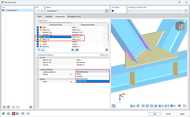
Za pomocą komponentu "Cięcie płyty" można ciąć blachy (np. blachy węzłowe, blachy środnika itp.). Dostępne są różne metody cięcia:
- Płaszczyzna: Cięcie jest wykonywane na powierzchni najbliższej płycie odniesienia.
- Powierzchnia: Wycinane są tylko przecinające się części płyt.
- Bryła ograniczająca: Najbardziej zewnętrzny wymiar, szerokość i wysokość, jest wycinany jako prostokąt.
- Otoczka wypukła: Zewnętrzna otoczka przekroju służy do przycinania płyty. Jeżeli w węzłach narożnych przekroju występują zaokrąglenia, cięcie jest do nich dostosowywane.
- 002452
- Ogólne informacje
- Projektowanie konstrukcji aluminiowych RFEM 6
- Projektowanie konstrukcji aluminiowych RSTAB 9
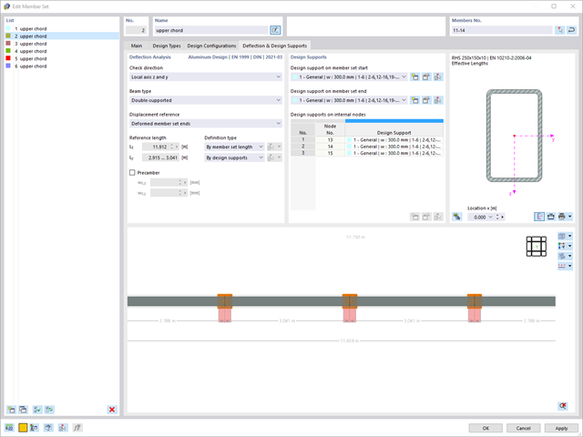
Program wykonuje za Ciebie dużo pracy. Na przykład kombinacje obciążeń lub wyników, które są niezbędne dla stanu granicznego użytkowalności, są generowane i obliczane w programie RFEM/RSTAB. Te sytuacje obliczeniowe można wybrać w rozszerzeniu Aluminium Design w celu przeprowadzenia analizy ugięcia. W zależności od wprowadzonej przechyłki i wybranego układu odniesienia program określa obliczone wartości deformacji w każdym punkcie pręta. Następnie są one porównywane z wartościami granicznymi.
W konfiguracji Stan graniczny użytkowalności można ustawić wartość graniczną, która ma być obserwowana dla odkształcenia dla każdego komponentu z osobna. Jako dopuszczalną wartość graniczną definiuje się maksymalne odkształcenie w zależności od długości odniesienia. Definiując podpory obliczeniowe, można segmentować komponenty. W ten sposób można automatycznie określić odpowiednią długość odniesienia dla każdego kierunku obliczeń.
To nie wszystko. W oparciu o położenie przypisanych podpór obliczeniowych program automatycznie umożliwia rozróżnienie belek i belek wspornikowych. W ten sposób określana jest odpowiednio wartość graniczna.
- 002453
- Ogólne informacje
- Projektowanie konstrukcji aluminiowych RFEM 6
- Projektowanie konstrukcji aluminiowych RSTAB 9
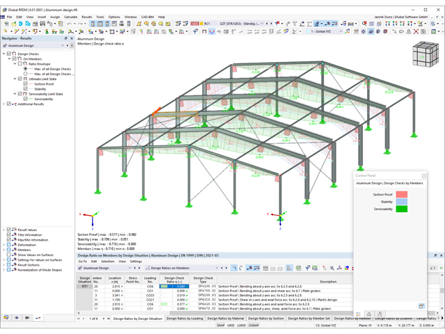
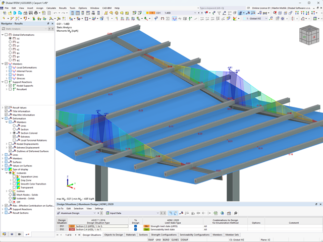
Obliczenia w stanie granicznym użytkowalności można znaleźć w tabelach wyników w rozszerzeniu do obliczeń dla aluminium. Są tam już w pełni zintegrowane. Istnieje możliwość uzyskania wyników obliczeń w każdym punkcie wymiarowanych prętów ze wszystkimi szczegółami. Można również użyć grafiki z wynikami współczynników obliczeniowych.
W razie potrzeby wszystkie tabele wyników i grafiki można uwzględnić jako część wyników obliczeń aluminium w globalnym raporcie wydruku programu RFEM/RSTAB. Program RFEM/RSTAB umożliwia również wyświetlanie i dokumentowanie wartości deformacji całej konstrukcji niezależnie od tego, czy jest to moduł dodatkowy.
Budowanie kamień na kamieniu ma długą tradycję w budownictwie. Rozszerzenie Projektowanie konstrukcji murowych dla RFEM umożliwia wymiarowanie konstrukcji murowych przy użyciu metody elementów skończonych. Rozszerzenie powstało w ramach projektu badawczego DDMaS - Digitalizacja wymiarowania konstrukcji murowych. Model materiałowy przedstawia nieliniowe zachowanie połączenia cegła-zaprawa w postaci modelowania w skali makro. Chcesz dowiedzieć się więcej?
- 002456
- Ogólne informacje
- Projektowanie konstrukcji aluminiowych RFEM 6
- Projektowanie konstrukcji aluminiowych RSTAB 9
Przy obliczaniu granicznego ugięcia należy wziąć pod uwagę określone długości odniesienia. Te długości odniesienia i sprawdzane segmenty można definiować niezależnie od siebie, w zależności od kierunku. W tym celu należy zdefiniować podpory obliczeniowe w węzłach pośrednich pręta i przypisać je do odpowiedniego kierunku dla analizy deformacji. Tworzy to segmenty, w których można uwzględnić przechyłkę dla każdego kierunku i segmentu.
_(1).png?mw=640&hash=415f7bbaf70e41679bb0106e1cf91eaa8c493ec9)
- Automatyczne generowanie modeli do analizy ES: rozszerzenie automatycznie tworzy w tle model elementów skończonych (ES) połączenia stalowego.
- Uwzględnienie wszystkich sił wewnętrznych: Obliczenia obejmują wszystkie siły wewnętrzne (N , Vy, Vz ,My, Mz, MT ) i nie są ograniczone do obciążeń płaskich.
- Automatyczne przenoszenie obciążeń: Wszystkie kombinacje obciążeń są automatycznie przenoszone do modelu analitycznego ES połączenia. Obciążenia są przenoszone bezpośrednio z programu RFEM, dzięki czemu ręczne wprowadzanie danych nie jest konieczne.
- Wydajne modelowanie: Rozszerzenie pozwala zaoszczędzić czas podczas modelowania złożonych sytuacji związanych z połączeniami. Utworzony model analityczny ES można również zapisać i wykorzystać do własnych szczegółowych analiz.
- Rozszerzalna biblioteka: Dostępna jest obszerna, rozszerzalna biblioteka zawierająca wstępnie zdefiniowane szablony połączeń stalowych.
- Szerokie zastosowanie: Rozszerzenie jest odpowiednie do tworzenia połączeń każdego typu i kształtu, jest kompatybilne z prawie wszystkimi przekrojami walcowanymi, spawanymi, złożonymi i cienkościennymi.

- 002109
- Ogólne informacje
- Optymalizacja i koszty | Szacowanie emisji CO2 RFEM 6
- Optymalizacja i koszty | Szacowanie emisji CO2 RSTAB 9
Masz pytania dotyczące programu? Optymalizacja konstrukcji w programach RFEM i RSTAB jest uzupełnieniem parametrycznego wprowadzania danych. Jest to proces równoległy, niezależny od rzeczywistych obliczeń modelu wraz ze wszystkimi jego zwykłymi definicjami obliczeń i obliczeń. Rozszerzenie zakłada, że model lub blok jest zbudowany w kontekście parametrycznym i jest kontrolowany przez globalne parametry kontrolne typu "optymalizacja". Dlatego te parametry kontrolne mają dolną i górną granicę oraz wielkość kroku w celu ograniczenia zakresu optymalizacji. Aby znaleźć optymalne wartości parametrów kontrolnych, należy określić kryterium optymalizacji (na przykład minimalny ciężar) przy wyborze metody optymalizacji (na przykład optymalizacja roju cząstek).
Oszacowanie kosztów i emisji CO2 można znaleźć już w definicjach materiałów. Obie opcje można aktywować osobno w każdej definicji materiału. Oszacowanie oparte jest na koszcie jednostkowym lub jednostkowej wartości emisji dla prętów, powierzchni oraz brył. W tym przypadku można wybrać, czy jednostki mają zostać podane według masy, objętości czy powierzchni.
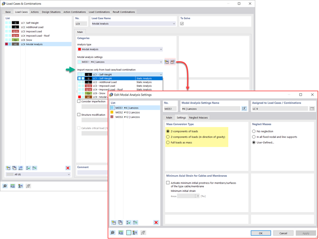
Dostępnych jest kilka opcji definiowania mas dla analizy modalnej. Masy od ciężaru własnego są uwzględniane automatycznie, natomiast obciążenia i masy można uwzględnić bezpośrednio w przypadku obciążenia typu analiza modalna. Potrzebujesz więcej opcji? Należy wybrać, czy obciążenia pełne mają być uwzględniane jako masy, składowe obciążenia w globalnym kierunku Z, czy tylko składowe obciążenia w kierunku siły ciężkości.
Program oferuje dodatkową lub alternatywną opcję importu mas: Ręczna definicja kombinacji obciążeń, począwszy od których masy są uwzględniane w analizie modalnej. Wybrałeś normę obliczeniową? Następnie można utworzyć sytuację obliczeniową typu Kombinacja mas sejsmicznych. W ten sposób program automatycznie oblicza sytuację masową dla analizy modalnej zgodnie z preferowaną normą obliczeniową. Innymi słowy: Program tworzy kombinację obciążeń na podstawie współczynników kombinacji wstępnie ustawionych dla wybranej normy. Zawiera on masy użyte do analizy modalnej.
- 002454
- Ogólne informacje
- Projektowanie konstrukcji aluminiowych RFEM 6
- Projektowanie konstrukcji aluminiowych RSTAB 9
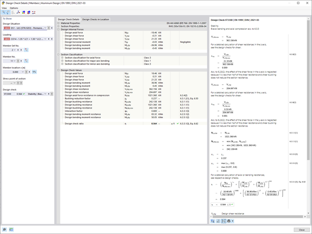
Czy bardzo to lubisz? My też! Z tego powodu wszystkie sprawdzenia dotyczące normy projektowej są wyświetlane w przejrzysty sposób. Dla każdej kontroli obliczeń należy zdefiniować kryterium wykorzystania. Szczegóły obliczeń, w których wartości wejściowe, wyniki pośrednie i wyniki końcowe są uporządkowane w sposób uporządkowany, są dostępne dla każdej kontroli obliczeń. Proces obliczeń wraz ze wszystkimi wzorami, normami i wynikami znajduje się w oknie informacyjnym, w którym wyświetlane są szczegóły obliczeń.

- 002108
- Ogólne informacje
- Optymalizacja i koszty | Szacowanie emisji CO2 RFEM 6
- Optymalizacja i koszty | Szacowanie emisji CO2 RSTAB 9
- Technologia sztucznej inteligencji (AI): Optymalizacja roju cząstek (PSO)
- Optymalizacja konstrukcji ze względu na minimalny ciężar lub deformację
- Możliwość zastosowania dowolnej liczby parametrów optymalizacyjnych
- Określanie zakresów zmiennych
- Optymalizacja przekrojów i materiałów
- Typy definicji parametrów
- Optymalizacja | Rosnąco, czyli optymalizacja | Malejąca
- Zastosowanie parametrycznych modeli i bloków
- Parametryzacja bloków w języku JavaScript na podstawie kodu
- Optymalizacja z uwzględnieniem wyników obliczeń
- Tabelaryczne przedstawienie najlepszych mutacji modelu
- Wyświetlanie w czasie rzeczywistym mutacji modelu w procesie optymalizacji
- Kalkulacja kosztów modelu dzięki zadanym cenom jednostkowym
- Określanie potencjału tworzenia efektu cieplarnianego (GWP-global warming potential) na etapie tworzenia modelu poprzez szacowanie równoważnej emisji CO2
- Określanie jednostkowych wskaźników zależnych od masy, objętości i powierzchni (cena i emisja CO2)

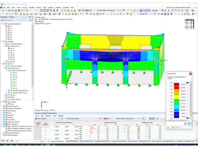
W przypadku analizy spektrum odpowiedzi modeli budynków można wyświetlić współczynniki wrażliwości dla kierunków poziomych według kondygnacji.
Dzięki tym kluczowym wartościom można zinterpretować wrażliwość na efekty stateczności.
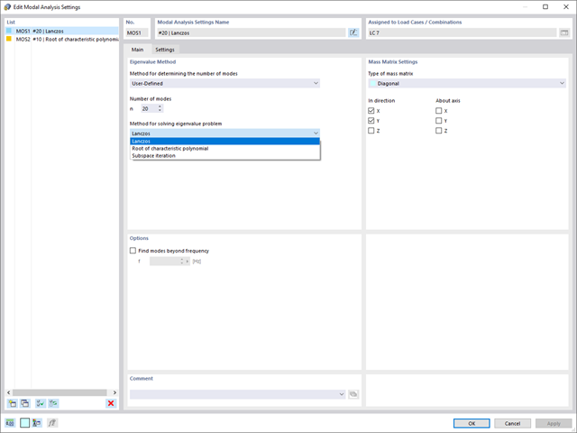
W programie RFEM dostępne są trzy wydajne solwery wartości własnych:
- pierwiastek wielomianu charakterystycznego
- Metoda Lanchosa
- iteracja podprzestrzeni
Z kolei program RSTAB oferuje dwa solwery wartości własnych:
- iteracja podprzestrzeni
- Metoda Powera z przesuniętą odwrotnością
Wybór solwera wartości własnych zależy przede wszystkim od rozmiaru modelu.

- 002110
- Ogólne informacje
- Optymalizacja i koszty | Szacowanie emisji CO2 RFEM 6
- Optymalizacja i koszty | Szacowanie emisji CO2 RSTAB 9
Istnieją dwie metody optymalizacji, dzięki którym można znaleźć optymalne wartości parametrów według kryterium ciężaru lub odkształcenia.
Najbardziej wydajną metodą o najkrótszym czasie obliczeń jest optymalizacja roju cząstek zbliżona do naturalnej (PSO). Czy słyszałeś lub czytałeś o tym? Ta technologia sztucznej inteligencji (AI) ma silną analogię do zachowania stad zwierząt szukających miejsca odpoczynku. W takich rojach można znaleźć wiele osób (por. rozwiązanie optymalizacyjne - na przykład waga), które lubią przebywać w grupie i podążać za ruchem grupy. Załóżmy, że każdy pręt roju musi zostać poddany spoczynkowi w optymalnym miejscu (por. najlepsze rozwiązanie - na przykład najniższa waga). Potrzeba ta wzrasta wraz ze zbliżaniem się do miejsca odpoczynku. Na zachowanie roju mają zatem wpływ również właściwości przestrzeni (por. wykres wyników).
Dlaczego wycieczka do biologii? Po prostu - proces PSO w RFEM lub RSTAB przebiega w podobny sposób. Proces obliczeń rozpoczyna się od wyniku optymalizacji poprzez losowe przypisanie parametrów, które mają zostać zoptymalizowane. Wielokrotnie określa nowe wyniki optymalizacji ze zróżnicowanymi wartościami parametrów, które opierają się na doświadczeniach z wcześniej przeprowadzonych mutacji modelu. Proces jest kontynuowany do momentu osiągnięcia określonej liczby możliwych mutacji modelu.
Jako alternatywa dla tej metody program oferuje również metodę przetwarzania wsadowego. Metoda ta ma na celu sprawdzenie wszystkich możliwych mutacji modelu poprzez losowe określanie wartości parametrów optymalizacji, aż do osiągnięcia określonej liczby możliwych mutacji modelu.
Po obliczeniu mutacji modelu obydwa warianty sprawdzają również odpowiednie aktywowane wyniki obliczeń rozszerzeń. Ponadto zapisuje on wariant z odpowiednim wynikiem optymalizacji i przypisaniem wartości parametrów optymalizacji, jeżeli wykorzystanie jest < 1.
Na podstawie odpowiednich sum poszczególnych materiałów można określić szacunkowe koszty całkowite i emisję. Na sumę materiałów składają się zależne od ciężaru, objętości i powierzchnie elementów prętowych, powierzchniowych i bryłowych.
- 002464
- Wyniki
- Projektowanie konstrukcji aluminiowych RFEM 6
- Projektowanie konstrukcji aluminiowych RSTAB 9
Jak zwykle, wprowadzasz układ i obliczasz siły wewnętrzne w programach RFEM i RSTAB. Masz nieograniczony dostęp do obszernych bibliotek materiałów i przekrojów. Czy wiesz, że za pomocą programu RSECTION można tworzyć przekroje ogólne? Oszczędza to dużo pracy.
Nie bój się'dodatkowych okien i chaosu przy wprowadzaniu danych! Dzieje się tak, ponieważ wymiarowanie aluminium jest w pełni zintegrowane z programami głównymi i automatycznie uwzględnia konstrukcję oraz istniejące wyniki obliczeń. Dalsze dane wejściowe dla obliczeń aluminium, takie jak długości efektywne, redukcje przekroju lub parametry obliczeniowe, można przypisać bezpośrednio do projektowanych obiektów. W wielu miejscach programu najlepiej jest użyć funkcji [Wskaż] do wyboru grafiki - w prosty i efektywny sposób.
- 002460
- Ogólne informacje
- Projektowanie konstrukcji aluminiowych RFEM 6
- Projektowanie konstrukcji aluminiowych RSTAB 9
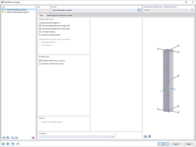
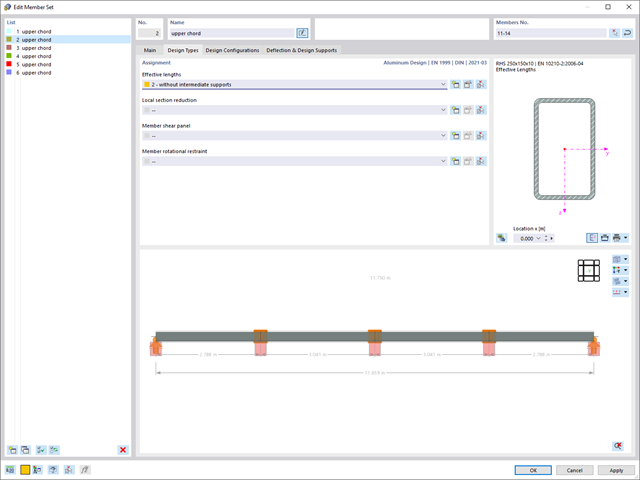
Należy upewnić się, że zdefiniowanie długości efektywnych w aluminiowym module dodatkowym jest warunkiem niezbędnym do przeprowadzenia analizy stateczności. W tym celu w oknie dialogowym należy zdefiniować podpory węzłowe i współczynniki długości efektywnej. Czy chcesz przejrzyście udokumentować podpory węzłowe i wynikające z nich segmenty wraz z powiązanym współczynnikiem długości efektywnej? W celu sprawdzenia wprowadzonych danych najlepiej jest użyć prezentacji graficznej w oknie roboczym programu RFEM/RSTAB. Oznacza to, że możesz zrozumieć projekt w dowolnym momencie i bez większego wysiłku.
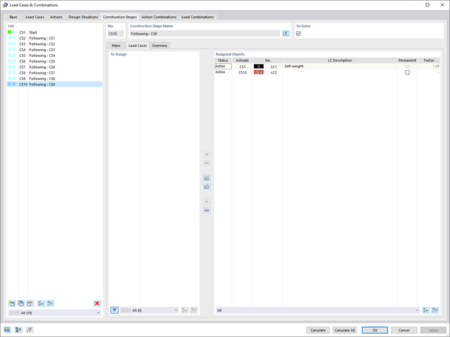
Czy udało Ci się utworzyć całą konstrukcję w programie RFEM? Dobrze, teraz można przypisać poszczególne elementy konstrukcyjne i przypadki obciążeń do odpowiednich etapów budowy. Na każdym etapie budowy można modyfikować na przykład definicje zwolnień prętów i podpór.
Pozwala to na modelowanie zmian konstrukcyjnych, na przykład podczas betonowania dźwigarów mostowych lub osiadania słupów. Przypadki obciążeń utworzone w programie RFEM należy następnie przydzielić do etapów budowy jako obciążenia stałe lub przejściowe.
Czy wiecie, że...? Kombinatoryka umożliwia nakładanie obciążeń stałych i przejściowych w kombinacjach obciążeń. W ten sposób można określić maksymalne siły wewnętrzne dla różnych pozycji dźwigu lub uwzględnić tymczasowe obciążenia montażowe dostępne tylko w jednym etapie budowy.
- 002141
- Ogólne informacje
- Projektowanie konstrukcji aluminiowych RFEM 6
- Projektowanie konstrukcji aluminiowych RSTAB 9
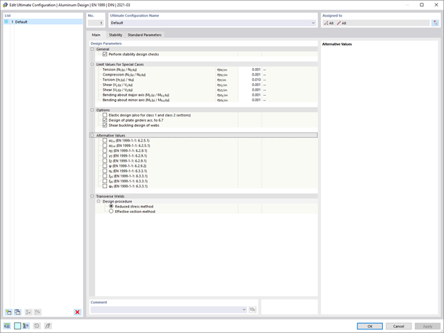
- Wymiarowanie elementów rozciąganych, ściskanych, zginanych, ścinanych, skręcanych i poddanych połączonemu działaniu tych sił wewnętrznych
- Obliczanie rozciągania z uwzględnieniem zredukowanej powierzchni przekroju (np. osłabienie z uwagi na otwory)
- Automatyczna klasyfikacja przekrojów w celu sprawdzenia wyboczenia lokalnego
- Siły wewnętrzne z obliczeń ze skręcaniem skrępowanym (7 stopni swobody) są uwzględniane w kontroli naprężeń zastępczych (obecnie nie dla normy ADM 2020)
- Wymiarowanie przekrojów klasy 4 o właściwościach przekroju efektywnego zgodnie z EN 1999-1-1 (dla przekrojów RSECTION wymagane są licencje dla przekrojów RSECTION i "Przekroje efektywne")
- Sprawdzenie wyboczenia przy ścinaniu z uwzględnieniem usztywnień poprzecznych
- 002451
- Ogólne informacje
- Projektowanie konstrukcji aluminiowych RFEM 6
- Projektowanie konstrukcji aluminiowych RSTAB 9
- Obliczanie ugięć i porównanie z normatywnymi lub ręcznie dostosowanymi wartościami granicznymi
- Uwzględnienie wygięcia wstępnego w analizie ugięcia
- W zależności od typu sytuacji obliczeniowej możliwe są różne wartości graniczne
- Ręczne dostosowywanie długości odniesienia i segmentacji według kierunku
- Obliczenia ugięć w odniesieniu do konstrukcji wyjściowej lub konstrukcji odkształconej
- Dalsze szczegółowe weryfikacje w zależności od wybranej normy obliczeniowej (np. weryfikacja drgań zgodnie z EN 1999-1-1, 7.2.3)
- Graficzne wyświetlanie wyników zintegrowane w programie RFEM/RSTAB, na przykład stopień wykorzystania wartości granicznej, odkształcenie lub ugięcie
- Pełna integracja wyników z raportem RFEM/RSTAB