42 Wyniki
Wyświetl wyniki:
Sortuj według:
- 002111
- Ogólne informacje
- Analiza naprężeniowo-odkształceniowa RFEM 6
- Analiza naprężeniowo-odkształceniowa RSTAB 9
- Ogólna analiza naprężeniowa
- Automatyczny import sił wewnętrznych z programu RFEM/RSTAB
- Graficzne i numeryczne przedstawianie naprężeń, odkształceń, luzu i stopni wykorzystania w pełni zintegrowane z RFEM/RSTAB
- Zdefiniowana przez użytkownika specyfikacja naprężenia granicznego
- Podsumowanie podobnych elementów konstrukcyjnych do obliczeń
- Szeroki zakres opcji umożliwiających dostosowywania sposobu wyświetlania wyników
- Przejrzyste tabele wyników dla szybkiego ich przeglądania po zakończeniu obliczeń
- Łatwa możliwość identyfikacji wyników dzięki w pełni udokumentowanej metodzie obliczeniowej wraz ze wszystkimi wzorami
- Wysoka wydajność pracy dzięki minimalnej ilości danych wejściowych
- Elastyczność dzięki szczegółowym opcjom ustawień dla podstawy i zakresu obliczeń
- Wyświetlanie szarej strefy dla nieistotnych zakresów wartości: Funkcja produktu "Analiza naprężeniowo-odkształceniowa z wyświetlaniem w szarej strefie"
- 002112
- Ogólne informacje
- Analiza naprężeniowo-odkształceniowa RFEM 6
- Analiza naprężeniowo-odkształceniowa RSTAB 9
- Optymalizacja przekroju
- Transfer zoptymalizowanych przekrojów do RFEM/RSTAB
- Wymiarowanie dowolnego przekroju cienkościennego z RSECTION
- Odwzorowanie wykresu naprężeń na przekroju
- Wyznaczanie naprężeń normalnych, ścinających i równoważnych
- Wyświetlanie składowych naprężeń dla poszczególnych typów sił wewnętrznych pręta
- Szczegółowe przedstawienie naprężeń we wszystkich punktach naprężeniowych
- Wyznaczanie największego Δσ dla każdego punktu naprężenia (na przykład do obliczeń zmęczenia)
- Wyświetlanie w kolorze naprężeń i stopni wykorzystania w celu szybkiego przeglądu stref krytycznych lub przewymiarowanych
- Wyświetlanie wykazów materiałów
- Wyznaczanie naprężeń głównych i podstawowych, naprężeń membranowych i stycznych oraz naprężeń zastępczych i zastępczych naprężeń membranowych
- Analiza naprężeń dla elementów konstrukcyjnych o dowolnym kształcie
- Obliczanie naprężeń zastępczych według różnych metod:
- Hipoteza energii odkształcenia (von Mises)
- Schubspannungshypothese (Tresca)
- Normalspannungshypothese (Rankine)
- Hauptdehnungshypothese (Bach)
- Możliwość optymalizacji grubości powierzchni i transferu danych do programu RFEM
- Ausgabe der Dehnungen
- Szczegółowe wyniki dla różnych składników naprężeń i stopni wykorzystania w tabelach i w grafice
- Filtermöglichkeit für Volumenkörper, Flächen, Linien und Knoten in Tabellen
- Querschubspannungen nach Mindlin, Kirchhoff oder freier Eingabe
- Spannungsauswertung für Schweißnähte an Verbindungslinien zwischen Flächen: Przejdź do funkcji produktu "Spoina liniowa"
- 002115
- Wyniki
- Analiza naprężeniowo-odkształceniowa RFEM 6
- Analiza naprężeniowo-odkształceniowa RSTAB 9
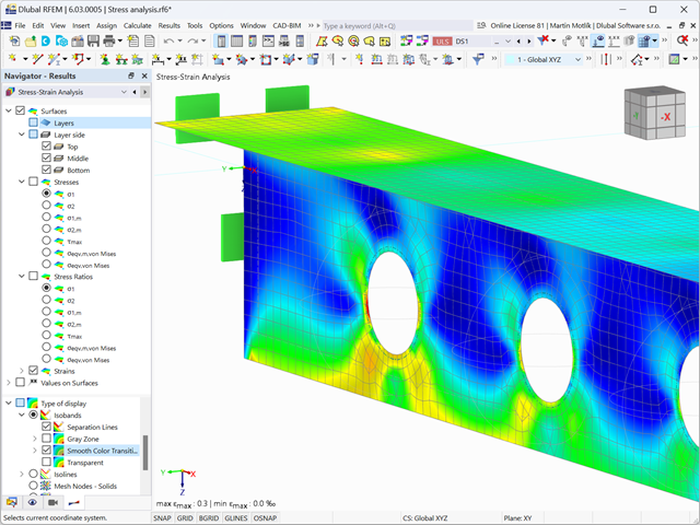
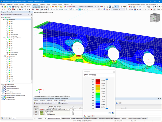
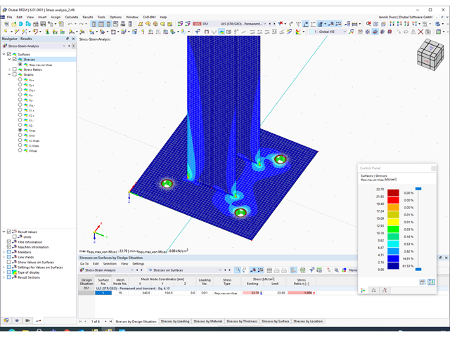
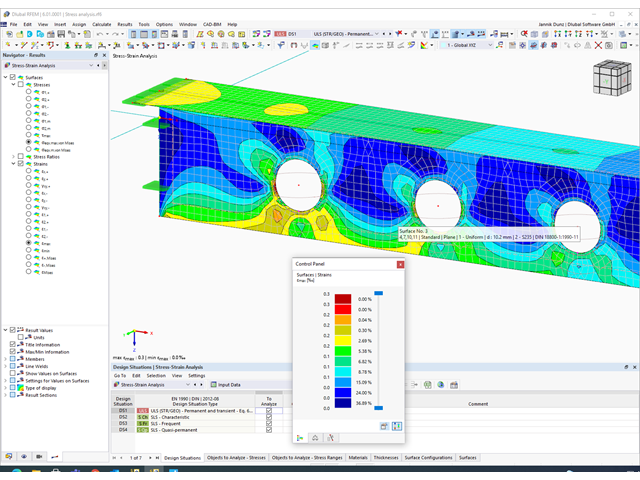
Po zakończeniu obliczeń wyniki są uporządkowane w sposób przejrzysty. W ten sposób program wyświetla maksymalne naprężenia i stopnie naprężeń posortowane według przekroju, pręta/powierzchni, bryły, zbioru prętów, położenia x itd. Oprócz wartości wyników w formie tabelarycznej rozszerzenie wyświetla również odpowiednią grafikę przekroju z punktami naprężeniowymi, wykresem naprężeń i wartościami. Stopień wykorzystania można odnieść do dowolnego rodzaju naprężenia. Aktualnie wybrana lokalizacja na elemencie zostanie wyróżniona na modelu analitycznym w programie RFEM/RSTAB.
Oprócz oceny tabelarycznej program oferuje jeszcze więcej. Naprężenia i stopnie wykorzystania można również sprawdzić graficznie na modelu w programie RFEM/RSTAB. Istnieje możliwość indywidualnego dostosowania kolorów i wartości.
Wyświetlanie wykresów wyników dla pręta lub zbioru prętów umożliwia dokładną ocenę. Dla każdego miejsca obliczeniowego można otworzyć odpowiednie okno dialogowe, w którym można sprawdzić odpowiednie do obliczeń właściwości przekroju i składowe naprężeń w dowolnym punkcie naprężeniowym. Na koniec istnieje możliwość wydrukowania odpowiedniej grafiki wraz ze wszystkimi szczegółami obliczeń.
- Realistyczne odwzorowanie interakcji między budynkiem a gruntem
- Realistyczne odwzorowanie oddziaływania poszczególnych fundamentów na siebie nawzajem
- Biblioteka parametrów gruntowych z możliwością rozszerzania
- Możliwość uwzględniania wielu próbek gruntu z różnych lokalizacji, także poza obrysem budynku
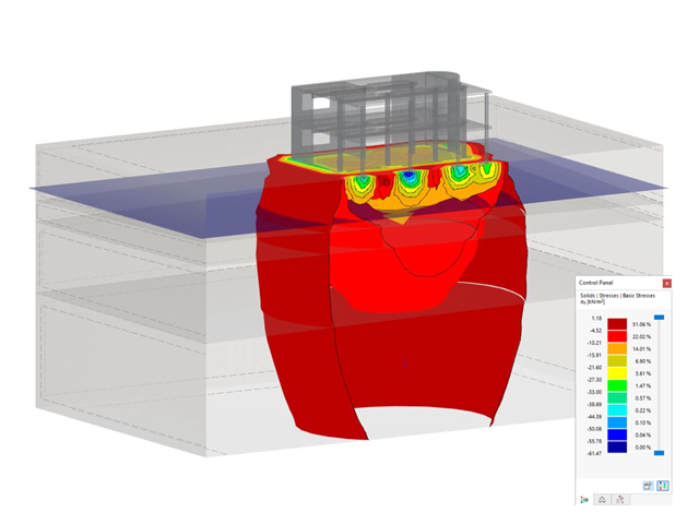
- Określanie osiadań oraz wykresów naprężeń w gruncie oraz ich prezentacja w formie graficznej i tabelarycznej

Wprowadzanie warstw gruntu dla potrzeb zadawania próbek gruntu odbywa się w przejrzystym oknie dialogowym. Odpowiadająca temu prezentacja graficzna zapewnia przejrzystość i ułatwia kontrolę wprowadzanych danych.
Rozszerzalna baza danych ułatwia wybór właściwości materiałowych dla gruntu. Dla realistycznego odwzorowania zachowania się materiału gruntowego można użyć modelu Mohra-Coulomba oraz model gruntu ze wzmocnieniem.
Można zdefiniować dowolną liczbę próbek i warstw gruntu. Grunt jest odwzorowany na podstawie wszystkich wprowadzonych próbek za pomocą brył 3D. Przypisanie do konstrukcji odbywa się za pomocą współrzędnych.
Zachowanie bryły gruntu jest obliczane za pomocą nieliniowej metody iteracyjnej. Obliczone naprężenia i osiadania są wyświetlane graficznie oraz w tabelach.
- Proste definiowanie etapów budowy konstrukcji w RFEM wraz z wizualizacją
- Dodawanie, usuwanie, modyfikowanie i reaktywacja elementów prętowych, powierzchniowych i bryłowych oraz ich właściwości (np. przeguby prętowe i liniowe, stopnie swobody dla podpór itp.)
- Ręczna oraz automatyczna kombinatoryka obciążeń na poszczególnych etapach budowy konstrukcji (np. w celu uwzględnienia obciążeń montażowych, tymczasowych urządzeń dźwigowych itp.)
- Uwzględnienie wpływów nieliniowych, takich jak uszkodzenie prętów rozciąganych lub nieliniowe zachowanie podpór
- Interakcja z innymi rozszerzeniami, takimi jak z. B. Nieliniowe zachowanie materiału, Stateczność konstrukcji, -rstab-9/additional-analyses/form-finding/form-finding itd.
- Wyświetlanie wyników w postaci numerycznej i graficznej dla poszczególnych etapów budowy
- Szczegółowy protokół wydruku wraz z dokumentacją wszystkich danych konstrukcyjnych i obciążeń dla każdego etapu budowy
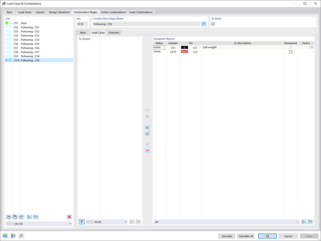
Czy udało Ci się utworzyć całą konstrukcję w programie RFEM? Dobrze, teraz można przypisać poszczególne elementy konstrukcyjne i przypadki obciążeń do odpowiednich etapów budowy. Na każdym etapie budowy można modyfikować na przykład definicje zwolnień prętów i podpór.
Pozwala to na modelowanie zmian konstrukcyjnych, na przykład podczas betonowania dźwigarów mostowych lub osiadania słupów. Przypadki obciążeń utworzone w programie RFEM należy następnie przydzielić do etapów budowy jako obciążenia stałe lub przejściowe.
Czy wiecie, że...? Kombinatoryka umożliwia nakładanie obciążeń stałych i przejściowych w kombinacjach obciążeń. W ten sposób można określić maksymalne siły wewnętrzne dla różnych pozycji dźwigu lub uwzględnić tymczasowe obciążenia montażowe dostępne tylko w jednym etapie budowy.
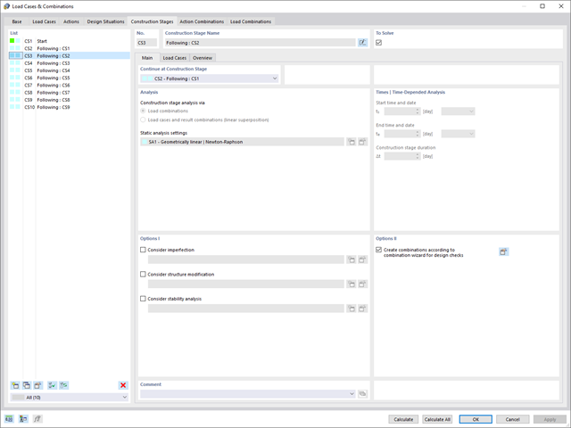
Jeżeli między idealnym układem a układem, który uległ deformacji z poprzedniego etapu budowy, pojawią się różnice w geometrii, są one porównywane w programie. Następujące po sobie kolejne etapy budowy obliczane są na bazie układu konstrukcyjnego z odkształceniami i obciążeniami wynikającymi z poprzednich etapu budowy. Obliczenia te są nieliniowe.
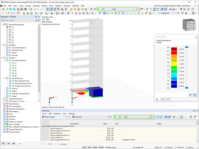
Czy obliczenia zakończyły się pomyślnie? Wyniki poszczególnych etapów budowy można teraz wyświetlać graficznie oraz w tabelach w programie RFEM. Ponadto program RFEM umożliwia uwzględnienie etapów budowy w kombinatoryce i uwzględnienie ich w dalszych obliczeniach.
_ENG.png?mw=640&hash=1053c9bef400e9f5361c9c3278f76a272fcc4ddf)
Czy aktywowałeś rozszerzenie Analiza historii czasowej (TDA)? Dobrze, teraz można dodawać dane czasowe do przypadków obciążeń. Po zdefiniowaniu początku i końca obciążenia, uwzględniany jest wpływ pełzania na końcu obciążenia. Program umożliwia modelowanie efektów pełzania w konstrukcjach szkieletowych i kratowych wykonanych z betonu zbrojonego.
W tym przypadku obliczenia są przeprowadzane nieliniowo zgodnie z modelem reologicznym (model Kelvina i Maxwella).
Czy obliczenia zakończyły się pomyślnie? Wyznaczone siły wewnętrzne można teraz wyświetlić w tabelach i grafice, a także uwzględnić w obliczeniach.

- 002108
- Ogólne informacje
- Optymalizacja i koszty | Szacowanie emisji CO2 RFEM 6
- Optymalizacja i koszty | Szacowanie emisji CO2 RSTAB 9
- Technologia sztucznej inteligencji (AI): Optymalizacja roju cząstek (PSO)
- Optymalizacja konstrukcji ze względu na minimalny ciężar lub deformację
- Możliwość zastosowania dowolnej liczby parametrów optymalizacyjnych
- Określanie zakresów zmiennych
- Optymalizacja przekrojów i materiałów
- Typy definicji parametrów
- Optymalizacja | Rosnąco, czyli optymalizacja | Malejąca
- Zastosowanie parametrycznych modeli i bloków
- Parametryzacja bloków w języku JavaScript na podstawie kodu
- Optymalizacja z uwzględnieniem wyników obliczeń
- Tabelaryczne przedstawienie najlepszych mutacji modelu
- Wyświetlanie w czasie rzeczywistym mutacji modelu w procesie optymalizacji
- Kalkulacja kosztów modelu dzięki zadanym cenom jednostkowym
- Określanie potencjału tworzenia efektu cieplarnianego (GWP-global warming potential) na etapie tworzenia modelu poprzez szacowanie równoważnej emisji CO2
- Określanie jednostkowych wskaźników zależnych od masy, objętości i powierzchni (cena i emisja CO2)

- 002109
- Ogólne informacje
- Optymalizacja i koszty | Szacowanie emisji CO2 RFEM 6
- Optymalizacja i koszty | Szacowanie emisji CO2 RSTAB 9
Masz pytania dotyczące programu? Optymalizacja konstrukcji w programach RFEM i RSTAB jest uzupełnieniem parametrycznego wprowadzania danych. Jest to proces równoległy, niezależny od rzeczywistych obliczeń modelu wraz ze wszystkimi jego zwykłymi definicjami obliczeń i obliczeń. Rozszerzenie zakłada, że model lub blok jest zbudowany w kontekście parametrycznym i jest kontrolowany przez globalne parametry kontrolne typu "optymalizacja". Dlatego te parametry kontrolne mają dolną i górną granicę oraz wielkość kroku w celu ograniczenia zakresu optymalizacji. Aby znaleźć optymalne wartości parametrów kontrolnych, należy określić kryterium optymalizacji (na przykład minimalny ciężar) przy wyborze metody optymalizacji (na przykład optymalizacja roju cząstek).
Oszacowanie kosztów i emisji CO2 można znaleźć już w definicjach materiałów. Obie opcje można aktywować osobno w każdej definicji materiału. Oszacowanie oparte jest na koszcie jednostkowym lub jednostkowej wartości emisji dla prętów, powierzchni oraz brył. W tym przypadku można wybrać, czy jednostki mają zostać podane według masy, objętości czy powierzchni.

- 002110
- Ogólne informacje
- Optymalizacja i koszty | Szacowanie emisji CO2 RFEM 6
- Optymalizacja i koszty | Szacowanie emisji CO2 RSTAB 9
Istnieją dwie metody optymalizacji, dzięki którym można znaleźć optymalne wartości parametrów według kryterium ciężaru lub odkształcenia.
Najbardziej wydajną metodą o najkrótszym czasie obliczeń jest optymalizacja roju cząstek zbliżona do naturalnej (PSO). Czy słyszałeś lub czytałeś o tym? Ta technologia sztucznej inteligencji (AI) ma silną analogię do zachowania stad zwierząt szukających miejsca odpoczynku. W takich rojach można znaleźć wiele osób (por. rozwiązanie optymalizacyjne - na przykład waga), które lubią przebywać w grupie i podążać za ruchem grupy. Załóżmy, że każdy pręt roju musi zostać poddany spoczynkowi w optymalnym miejscu (por. najlepsze rozwiązanie - na przykład najniższa waga). Potrzeba ta wzrasta wraz ze zbliżaniem się do miejsca odpoczynku. Na zachowanie roju mają zatem wpływ również właściwości przestrzeni (por. wykres wyników).
Dlaczego wycieczka do biologii? Po prostu - proces PSO w RFEM lub RSTAB przebiega w podobny sposób. Proces obliczeń rozpoczyna się od wyniku optymalizacji poprzez losowe przypisanie parametrów, które mają zostać zoptymalizowane. Wielokrotnie określa nowe wyniki optymalizacji ze zróżnicowanymi wartościami parametrów, które opierają się na doświadczeniach z wcześniej przeprowadzonych mutacji modelu. Proces jest kontynuowany do momentu osiągnięcia określonej liczby możliwych mutacji modelu.
Jako alternatywa dla tej metody program oferuje również metodę przetwarzania wsadowego. Metoda ta ma na celu sprawdzenie wszystkich możliwych mutacji modelu poprzez losowe określanie wartości parametrów optymalizacji, aż do osiągnięcia określonej liczby możliwych mutacji modelu.
Po obliczeniu mutacji modelu obydwa warianty sprawdzają również odpowiednie aktywowane wyniki obliczeń rozszerzeń. Ponadto zapisuje on wariant z odpowiednim wynikiem optymalizacji i przypisaniem wartości parametrów optymalizacji, jeżeli wykorzystanie jest < 1.
Na podstawie odpowiednich sum poszczególnych materiałów można określić szacunkowe koszty całkowite i emisję. Na sumę materiałów składają się zależne od ciężaru, objętości i powierzchnie elementów prętowych, powierzchniowych i bryłowych.

- Definiowanie naprężeń na przykładzie sprężysto-plastycznego modelu materiałowego
- Wymiarowanie murowych konstrukcji tarczowych na ściskanie i ścinanie na modelu budynku lub na pojedynczym modelu
- Automatyczne określanie sztywności przegubu ściana-płyta
- Obszerna baza danych materiałów o prawie wszystkich kombinacjach kamienia i zapraw dostępnych na rynku austriackim (asortyment jest stale poszerzany, również dla innych krajów)
- Automatyczne określanie wartości materiałów zgodnie z Eurokodem 6 (ÖN EN 1996‑X)
- Możliwość przeprowadzenia analizy pushover
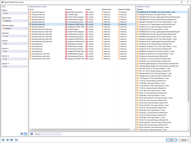
Konstrukcję wprowadza się i modeluje się bezpośrednio w programie RFEM. Model materiałowy muru można połączyć ze wszystkimi popularnymi rozszerzeniami dla programu RFEM. Umożliwia to projektowanie całych modeli budynków w połączeniu z murem.
Program automatycznie określa wszystkie parametry wymagane do obliczeń na podstawie wprowadzonych danych materiału. Następnie generowane są krzywe naprężenie-odkształcenie dla każdego elementu skończonego.
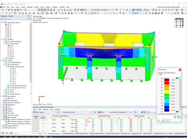
Czy projekt zakończył się sukcesem? Następnie po prostu usiądź i zrelaksuj się. Również tutaj można korzystać z licznych funkcji programu RFEM. Program podaje maksymalne naprężenia powierzchni murowanych, dzięki czemu można szczegółowo wyświetlić wyniki w każdym punkcie siatki ES.
Ponadto można wstawiać przekroje w celu przeprowadzenia szczegółowej analizy poszczególnych obszarów. Na podstawie przedstawionych obszarów uplastycznienia można oszacować zarysowania w murze.

- 002161
- Ogólne informacje
- Optymalizacja i koszty | Szacowanie emisji CO2 RFEM 6
- Optymalizacja i koszty | Szacowanie emisji CO2 RSTAB 9
Obie metody optymalizacji mają jedną wspólną cechę. Na końcu procesu wyświetlają listę wariacji modelu na podstawie przechowywanych danych. Można tu znaleźć szczegóły na temat wyniku decydującego dla optymalizacji i odpowiadające mu wartości parametrów. Lista jest zorganizowana w porządku malejącym. Zakładane najlepsze rozwiązanie znajduje się na górze. W takim przypadku wynik optymalizacji wraz z wyznaczoną wartością jest najbardziej zbliżony do kryterium optymalizacji. Wszystkie dodatkowe wyniki pokazują wykorzystanie < 1. Ponadto, po zakończeniu analizy, program dostosuje wartości na globalnej liście parametrów, aby odpowiadały tym dla optymalnego rozwiązania.
W oknach dialogowych materiałów znajdują się dodatkowe zakładki "Oszacowanie kosztów" i "Oszacowanie emisji CO2". Tutaj wyświetlane są indywidualne szacunkowe sumy przydzielonych prętów, powierzchni i objętości na jednostkę masy, objętości i powierzchni. Dodatkowo zakładki te podają całkowity koszt i emisję wszystkich przydzielonych do konstrukcji materiałów. Zapewnia to dobry przegląd projektu.
W porównaniu z modułem dodatkowym RF-/STAGES (RFEM 5) do rozszerzenia Analiza etapów budowy (CSA) dla programu RFEM 6 dodano następujące nowe funkcje:
- Uwzględnienie etapów budowy na poziomie programu RFEM
- Integracja analizy etapu budowy z kombinatoryką w programie RFEM
- Wprowadzono podparcie dla dodatkowych elementów konstrukcyjnych, takich jak przeguby liniowe
- Analiza alternatywnych procesów konstrukcyjnych w modelu
- Ponowna aktywacja elementów konstrukcyjnych
W porównaniu z modułem dodatkowym RF-SOILIN (RFEM 5) do rozszerzenia Analiza geotechniczna dla programu RFEM 6 dodano następujące nowe funkcje:
- Tworzenie warstwowego gruntu jako modelu 3D z całości zdefiniowanych próbek gruntu
- Symulacja gruntu zgodnie z teorią Mohra-Coulomba
- Graficzne i tabelaryczne przedstawienie naprężeń i odkształceń na dowolnej głębokości gruntu
- Optymalne uwzględnienie interakcji gruntu i konstrukcji na podstawie modelu ogólnego
- 002169
- Ogólne informacje
- Analiza naprężeniowo-odkształceniowa RFEM 6
- Analiza naprężeniowo-odkształceniowa RSTAB 9
W porównaniu z modułem dodatkowym RF-/STEEL (RFEM 5/RSTAB 8) do rozszerzenia Analiza naprężeniowo-odkształceniowa dla programu RFEM 6/RSTAB 9 dodano następujące nowe funkcje:
- Możliwość analizy prętów, powierzchni, brył, spoin (połączenia spawane liniowo między dwiema i trzema powierzchniami z późniejszym obliczaniem naprężeń)
- Wyświetlanie naprężeń, stopni naprężeń, zakresów naprężeń i odkształceń
- Naprężenie graniczne w zależności od przydzielonego materiału lub danych wejściowych zdefiniowanych przez użytkownika
- Indywidualne określenie wyników do obliczeń poprzez dowolnie przydzielane typów ustawień
- Szczegóły dla wyników niemodalnych z wyświetlaniem przygotowanego wzoru i dodatkowym wyświetlaniem wyników na poziomie przekroju prętów
- Możliwość wygenerowania zastosowanych wzorów do kontroli obliczeń

Dla każdego przypadku obciążenia można wyświetlić odkształcenia w czasie końcowym.
Wyniki te są również dokumentowane w protokole wydruku programów RFEM i RSTAB. Zawartość protokołu i jego zakres można wybrać specjalnie dla poszczególnych warunków projektowych.
Budowanie kamień na kamieniu ma długą tradycję w budownictwie. Rozszerzenie Projektowanie konstrukcji murowych dla RFEM umożliwia wymiarowanie konstrukcji murowych przy użyciu metody elementów skończonych. Rozszerzenie powstało w ramach projektu badawczego DDMaS - Digitalizacja wymiarowania konstrukcji murowych. Model materiałowy przedstawia nieliniowe zachowanie połączenia cegła-zaprawa w postaci modelowania w skali makro. Chcesz dowiedzieć się więcej?

- 002232
- Ogólne informacje
- Optymalizacja i koszty | Szacowanie emisji CO2 RFEM 6
- Optymalizacja i koszty | Szacowanie emisji CO2 RSTAB 9
Możesz być pewien, że koszty są ważnym czynnikiem w planowaniu konstrukcyjnym każdego projektu. Należy również przestrzegać przepisów dotyczących szacowania emisji. Dwuczęściowe rozszerzenie Optymalizacja i koszty/Szacowanie emisji CO2 ułatwia odnalezienie się w gąszczu norm i opcji. Wykorzystuje technologię sztucznej inteligencji (AI) optymalizacji rojem cząstek (PSO) w celu znalezienia odpowiednich parametrów dla sparametryzowanych modeli i bloków, które zagwarantują zgodność ze zwykłymi kryteriami optymalizacji. Ponadto, rozszerzenie oszacowuje koszty modelu lub emisję CO2 poprzez określenie kosztów jednostkowych lub emisji jednostkowej dla materiałów zdefiniowanych w modelu konstrukcyjnym. Dzięki temu rozszerzeniu jesteś po bezpiecznej stronie.
Dzięki rozszerzeniu Analiza historii czasowej (TDA) można uwzględnić zmienne w czasie zachowanie materiału w przypadku prętów i powierzchni. Długotrwałe efekty, takie jak pełzanie, skurcz i starzenie, mogą wpływać na rozkład sił wewnętrznych, w zależności od konstrukcji. Darauf bereiten Sie sich mit diesem Add-On optimal vor.
.png?mw=640&hash=25998fe3470f8e1c154828f202ad6a728b30f00a)
Czy wiecie, że...? Do obliczeń konstrukcji murowych w programie RFEM zaimplementowano nieliniowy model materiałowy. Opiera się ona na podejściu Lourenco, złożonej powierzchni plastyczności powierzchni według RANKINE'A i HILLA. Model ten umożliwia opisywanie i modelowanie konstrukcyjnego zachowania muru oraz różnych mechanizmów uszkodzenia.
Parametry graniczne dobrano tak, aby zastosowane krzywe projektowe odpowiadały normatywnej krzywej projektowej.
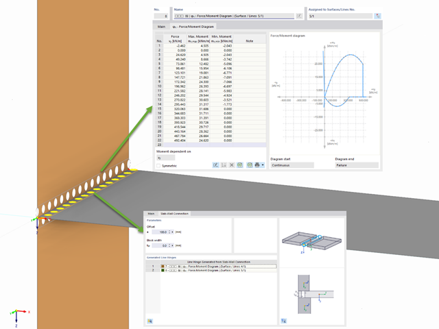
Program RFEM umożliwia wykorzystanie specjalnego przegubu liniowego do modelowania specjalnych właściwości połączenia między płytą żelbetową a ścianą murowaną. Ogranicza to przenoszone siły połączenia w zależności od określonej geometrii. Zgadnij dobrze: Oznacza to, że materiał nie może być przeciążony.
Program tworzy wykresy interakcji, które są stosowane automatycznie. Reprezentują one różne sytuacje geometryczne i można je wykorzystać do określenia prawidłowej sztywności.
.png?mw=640&hash=8b43c740f4a91092df759928a6ee21f06f78f8cc)
Obliczenia konstrukcji murowej są przeprowadzane zgodnie z prawem nieliniowo-plastycznym. Jeżeli obciążenie w dowolnym punkcie jest większe niż możliwe obciążenie, w układzie ma miejsce redystrybucja. Ma to na celu proste odtworzenie równowagi sił. Po pomyślnym zakończeniu obliczeń przeprowadzana jest analiza stateczności.
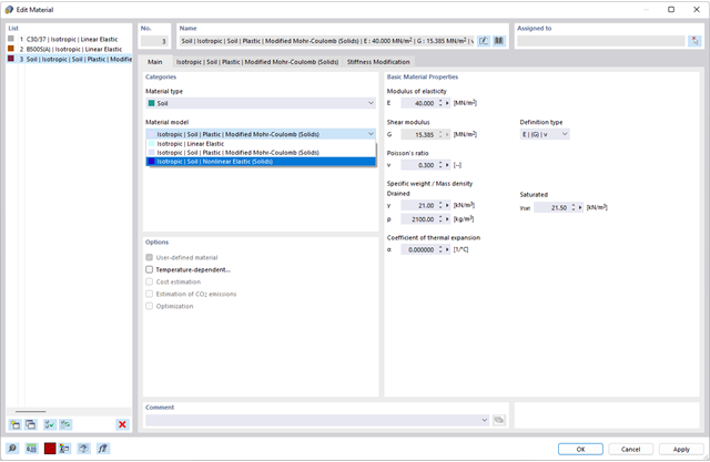
Czy chcesz modelować i analizować zachowanie bryły gruntowej? Aby to zapewnić, w programie RFEM zaimplementowano odpowiednie modele materiałowe.
Można użyć zmodyfikowanego modelu Mohra-Coulomba z liniowo-sprężystym modelem idealnie plastycznym lub nieliniowo sprężystym modelem z edometryczną relacją naprężenie-odkształcenie. Kryterium graniczne, które opisuje przejście od obszaru sprężystości do obszaru płynięcia plastycznego, jest zdefiniowane według Mohra-Coulomba.
Wprowadzenie i modelowanie bryły gruntowej bezpośrednio w programie RFEM. Modele materiałów gruntowych można łączyć ze wszystkimi popularnymi rozszerzeniami dla programu RFEM.
Umożliwia to łatwą analizę całych modeli z pełną prezentacją interakcji grunt-konstrukcja.
Wszystkie parametry wymagane do obliczeń są określane automatycznie na podstawie wprowadzonych danych materiałowych. Następnie program generuje krzywe naprężenie-odkształcenie dla każdego elementu ES.