21 Wyniki
Wyświetl wyniki:
Sortuj według:
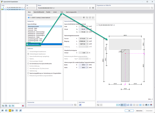
W rozszerzeniu Analiza etapów budowy (CSA) można używać przekrojów złożonych, dzięki zastosowaniu przekrojów etapowanych. Ten typ przekroju umożliwia aktywację lub dezaktywację poszczególnych części przekroju typu "Parametryczny - Masywny II" na poszczególnych etapach budowy.

W przypadku analizy spektrum odpowiedzi modeli budynków można wyświetlić współczynniki wrażliwości dla kierunków poziomych według kondygnacji.
Dzięki tym kluczowym wartościom można zinterpretować wrażliwość na efekty stateczności.
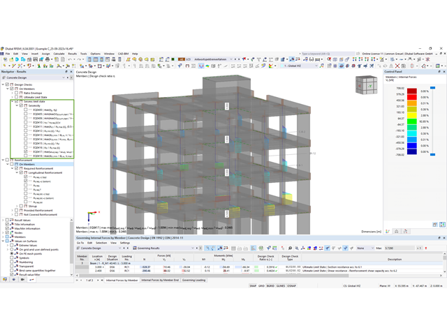
W rozszerzeniu Projektowanie konstrukcji betonowych można przeprowadzać obliczenia sejsmiczne dla prętów żelbetowych zgodnie z EC 8. Są to między innymi następujące funkcje:
- Konfiguracje obliczeń sejsmicznych
- Rozróżnianie klas ciągliwości DCL, DCM, DCH
- Możliwość przeniesienia współczynnika odpowiedzi z analizy dynamicznej
- Sprawdzenie wartości granicznej współczynnika odpowiedzi
- Weryfikacja nośności dla "Wytrzymały słup - słaba belka"
- Uszczegółowienie i reguły szczególne dla współczynnika ciągliwości krzywizny
- Uszczegółowienie i reguły szczególne dla ciągliwości lokalnej

- 002232
- Ogólne informacje
- Optymalizacja i koszty | Szacowanie emisji CO2 RFEM 6
- Optymalizacja i koszty | Szacowanie emisji CO2 RSTAB 9
Możesz być pewien, że koszty są ważnym czynnikiem w planowaniu konstrukcyjnym każdego projektu. Należy również przestrzegać przepisów dotyczących szacowania emisji. Dwuczęściowe rozszerzenie Optymalizacja i koszty/Szacowanie emisji CO2 ułatwia odnalezienie się w gąszczu norm i opcji. Wykorzystuje technologię sztucznej inteligencji (AI) optymalizacji rojem cząstek (PSO) w celu znalezienia odpowiednich parametrów dla sparametryzowanych modeli i bloków, które zagwarantują zgodność ze zwykłymi kryteriami optymalizacji. Ponadto, rozszerzenie oszacowuje koszty modelu lub emisję CO2 poprzez określenie kosztów jednostkowych lub emisji jednostkowej dla materiałów zdefiniowanych w modelu konstrukcyjnym. Dzięki temu rozszerzeniu jesteś po bezpiecznej stronie.

- 002165
- Ogólne informacje
- Skręcanie skrępowane (7 stopni swobody) RFEM 6
- Skręcanie skrępowane (7 stopni swobody) RSTAB 9
W porównaniu z modułem dodatkowym RF-/STEEL Warping Torsion (RFEM 5/RSTAB 8) do rozszerzenia Skręcanie skrępowane (7 DOF) dla programu RFEM 6/RSTAB 9 dodano następujące nowe funkcje:
- Pełna integracja ze środowiskiem RFEM 6 i RSTAB 9
- Siódmy stopień swobody jest bezpośrednio uwzględniany w obliczeniach prętów w programie RFEM/RSTAB na całym układzie
- Nie ma już potrzeby definiowania warunków podparcia lub sztywności sprężystej do obliczeń w uproszczonym układzie zastępczym
- Możliwość łączenia z innymi rozszerzeniami, na przykład do obliczania obciążeń krytycznych dla wyboczenia skrętnego i zwichrzenia z analizą stateczności
- Brak ograniczeń dla stalowych przekrojów cienkościennych (możliwe jest również obliczenie momentu krytycznego, na przykład dla belek o masywnych przekrojach drewnianych)
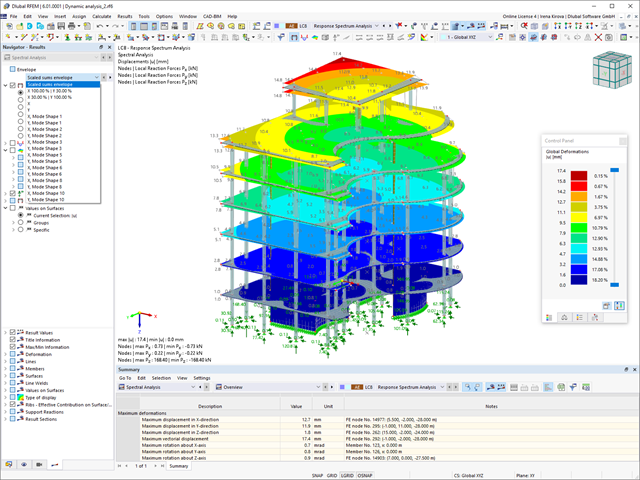
W porównaniu z modułem dodatkowym RF-/DYNAM Pro-Equivalent Loads (RFEM 5/RSTAB 8) do rozszerzenia Analiza spektrum odpowiedzi dla programu RFEM 6/RSTAB 9 dodano następujące nowe funkcje:
- Spektrum odpowiedzi z wielu norm (EN 1998, DIN 4149, IBC 2018 itd.)
- Spektrum odpowiedzi zdefiniowane przez użytkownika lub wygenerowane z akcelerogramów
- Możliwość zadania kierunkowego spektrum odpowiedzi
- Aby zapewnić przejrzystość wyniki są przechowywane łącznie, w jednym przypadku obciążenia, w ramach którego dostępne są różne poziomy wyświetlania
- Wpływ przypadkowych oddziaływań skręcających może być uwzględniany automatycznie
- Automatyczne kombinacje obciążeń sejsmicznych z innymi przypadkami obciążeń, możliwe do wykorzystania w wyjątkowej sytuacji obliczeniowej
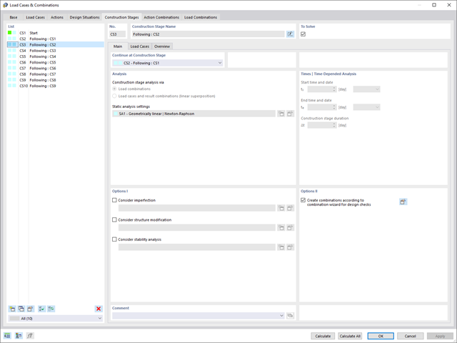
W porównaniu z modułem dodatkowym RF-/STAGES (RFEM 5) do rozszerzenia Analiza etapów budowy (CSA) dla programu RFEM 6 dodano następujące nowe funkcje:
- Uwzględnienie etapów budowy na poziomie programu RFEM
- Integracja analizy etapu budowy z kombinatoryką w programie RFEM
- Wprowadzono podparcie dla dodatkowych elementów konstrukcyjnych, takich jak przeguby liniowe
- Analiza alternatywnych procesów konstrukcyjnych w modelu
- Ponowna aktywacja elementów konstrukcyjnych

- 002108
- Ogólne informacje
- Optymalizacja i koszty | Szacowanie emisji CO2 RFEM 6
- Optymalizacja i koszty | Szacowanie emisji CO2 RSTAB 9
- Technologia sztucznej inteligencji (AI): Optymalizacja roju cząstek (PSO)
- Optymalizacja konstrukcji ze względu na minimalny ciężar lub deformację
- Możliwość zastosowania dowolnej liczby parametrów optymalizacyjnych
- Określanie zakresów zmiennych
- Optymalizacja przekrojów i materiałów
- Typy definicji parametrów
- Optymalizacja | Rosnąco, czyli optymalizacja | Malejąca
- Zastosowanie parametrycznych modeli i bloków
- Parametryzacja bloków w języku JavaScript na podstawie kodu
- Optymalizacja z uwzględnieniem wyników obliczeń
- Tabelaryczne przedstawienie najlepszych mutacji modelu
- Wyświetlanie w czasie rzeczywistym mutacji modelu w procesie optymalizacji
- Kalkulacja kosztów modelu dzięki zadanym cenom jednostkowym
- Określanie potencjału tworzenia efektu cieplarnianego (GWP-global warming potential) na etapie tworzenia modelu poprzez szacowanie równoważnej emisji CO2
- Określanie jednostkowych wskaźników zależnych od masy, objętości i powierzchni (cena i emisja CO2)

- 002109
- Ogólne informacje
- Optymalizacja i koszty | Szacowanie emisji CO2 RFEM 6
- Optymalizacja i koszty | Szacowanie emisji CO2 RSTAB 9
Masz pytania dotyczące programu? Optymalizacja konstrukcji w programach RFEM i RSTAB jest uzupełnieniem parametrycznego wprowadzania danych. Jest to proces równoległy, niezależny od rzeczywistych obliczeń modelu wraz ze wszystkimi jego zwykłymi definicjami obliczeń i obliczeń. Rozszerzenie zakłada, że model lub blok jest zbudowany w kontekście parametrycznym i jest kontrolowany przez globalne parametry kontrolne typu "optymalizacja". Dlatego te parametry kontrolne mają dolną i górną granicę oraz wielkość kroku w celu ograniczenia zakresu optymalizacji. Aby znaleźć optymalne wartości parametrów kontrolnych, należy określić kryterium optymalizacji (na przykład minimalny ciężar) przy wyborze metody optymalizacji (na przykład optymalizacja roju cząstek).
Oszacowanie kosztów i emisji CO2 można znaleźć już w definicjach materiałów. Obie opcje można aktywować osobno w każdej definicji materiału. Oszacowanie oparte jest na koszcie jednostkowym lub jednostkowej wartości emisji dla prętów, powierzchni oraz brył. W tym przypadku można wybrać, czy jednostki mają zostać podane według masy, objętości czy powierzchni.

- 002110
- Ogólne informacje
- Optymalizacja i koszty | Szacowanie emisji CO2 RFEM 6
- Optymalizacja i koszty | Szacowanie emisji CO2 RSTAB 9
Istnieją dwie metody optymalizacji, dzięki którym można znaleźć optymalne wartości parametrów według kryterium ciężaru lub odkształcenia.
Najbardziej wydajną metodą o najkrótszym czasie obliczeń jest optymalizacja roju cząstek zbliżona do naturalnej (PSO). Czy słyszałeś lub czytałeś o tym? Ta technologia sztucznej inteligencji (AI) ma silną analogię do zachowania stad zwierząt szukających miejsca odpoczynku. W takich rojach można znaleźć wiele osób (por. rozwiązanie optymalizacyjne - na przykład waga), które lubią przebywać w grupie i podążać za ruchem grupy. Załóżmy, że każdy pręt roju musi zostać poddany spoczynkowi w optymalnym miejscu (por. najlepsze rozwiązanie - na przykład najniższa waga). Potrzeba ta wzrasta wraz ze zbliżaniem się do miejsca odpoczynku. Na zachowanie roju mają zatem wpływ również właściwości przestrzeni (por. wykres wyników).
Dlaczego wycieczka do biologii? Po prostu - proces PSO w RFEM lub RSTAB przebiega w podobny sposób. Proces obliczeń rozpoczyna się od wyniku optymalizacji poprzez losowe przypisanie parametrów, które mają zostać zoptymalizowane. Wielokrotnie określa nowe wyniki optymalizacji ze zróżnicowanymi wartościami parametrów, które opierają się na doświadczeniach z wcześniej przeprowadzonych mutacji modelu. Proces jest kontynuowany do momentu osiągnięcia określonej liczby możliwych mutacji modelu.
Jako alternatywa dla tej metody program oferuje również metodę przetwarzania wsadowego. Metoda ta ma na celu sprawdzenie wszystkich możliwych mutacji modelu poprzez losowe określanie wartości parametrów optymalizacji, aż do osiągnięcia określonej liczby możliwych mutacji modelu.
Po obliczeniu mutacji modelu obydwa warianty sprawdzają również odpowiednie aktywowane wyniki obliczeń rozszerzeń. Ponadto zapisuje on wariant z odpowiednim wynikiem optymalizacji i przypisaniem wartości parametrów optymalizacji, jeżeli wykorzystanie jest < 1.
Na podstawie odpowiednich sum poszczególnych materiałów można określić szacunkowe koszty całkowite i emisję. Na sumę materiałów składają się zależne od ciężaru, objętości i powierzchnie elementów prętowych, powierzchniowych i bryłowych.

- 002161
- Ogólne informacje
- Optymalizacja i koszty | Szacowanie emisji CO2 RFEM 6
- Optymalizacja i koszty | Szacowanie emisji CO2 RSTAB 9
Obie metody optymalizacji mają jedną wspólną cechę. Na końcu procesu wyświetlają listę wariacji modelu na podstawie przechowywanych danych. Można tu znaleźć szczegóły na temat wyniku decydującego dla optymalizacji i odpowiadające mu wartości parametrów. Lista jest zorganizowana w porządku malejącym. Zakładane najlepsze rozwiązanie znajduje się na górze. W takim przypadku wynik optymalizacji wraz z wyznaczoną wartością jest najbardziej zbliżony do kryterium optymalizacji. Wszystkie dodatkowe wyniki pokazują wykorzystanie < 1. Ponadto, po zakończeniu analizy, program dostosuje wartości na globalnej liście parametrów, aby odpowiadały tym dla optymalnego rozwiązania.
W oknach dialogowych materiałów znajdują się dodatkowe zakładki "Oszacowanie kosztów" i "Oszacowanie emisji CO2". Tutaj wyświetlane są indywidualne szacunkowe sumy przydzielonych prętów, powierzchni i objętości na jednostkę masy, objętości i powierzchni. Dodatkowo zakładki te podają całkowity koszt i emisję wszystkich przydzielonych do konstrukcji materiałów. Zapewnia to dobry przegląd projektu.
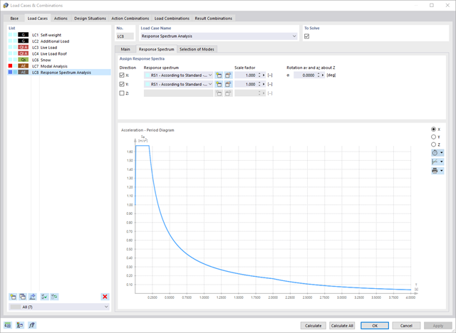
Oprogramowanie do analizy statyczno-wytrzymałościowej firmy Dlubal wykonuje wiele pracy za Ciebie. Program sugeruje zgodnie z regułami parametry wejściowe, istotne dla wybranych norm. Ponadto można ręcznie wprowadzić spektra odpowiedzi.
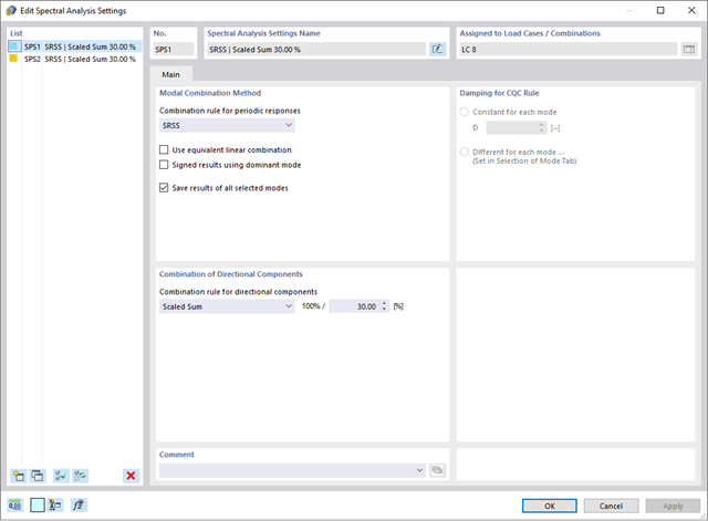
Przypadki obciążeń typu Analiza spektrum odpowiedzi określają kierunek, w którym działają spektra odpowiedzi oraz które wartości własne konstrukcji są istotne dla analizy. W ustawieniach analizy spektralnej można zdefiniować szczegóły dotyczące reguł kombinacji, tłumienia (jeśli ma zastosowanie) i przyspieszenia okresu zerowego (ZPA).
Czy wiecie, że...? Równoważne obciążenia statyczne generowane są oddzielnie dla każdej miarodajnej postaci drgań własnych oraz kierunku wzbudzenia. Obciążenia te są zapisywane w przypadku obciążenia typu Analiza spektrum odpowiedzi, a program RFEM/RSTAB przeprowadza liniową analizę statyczną.
Przypadki obciążeń typu Analiza spektrum odpowiedzi zawierają wygenerowane obciążenia równoważne. Po pierwsze, udziały modalne muszą zostać nałożone na siebie z regułą SRSS lub CQC. W takim przypadku można wykorzystać wyniki podpisane na podstawie dominującego kształtu drgań.
Następnie składowe kierunkowe oddziaływań sejsmicznych są łączone z regułą SRSS lub regułą 100%/30%.
- Proste definiowanie etapów budowy konstrukcji w RFEM wraz z wizualizacją
- Dodawanie, usuwanie, modyfikowanie i reaktywacja elementów prętowych, powierzchniowych i bryłowych oraz ich właściwości (np. przeguby prętowe i liniowe, stopnie swobody dla podpór itp.)
- Ręczna oraz automatyczna kombinatoryka obciążeń na poszczególnych etapach budowy konstrukcji (np. w celu uwzględnienia obciążeń montażowych, tymczasowych urządzeń dźwigowych itp.)
- Uwzględnienie wpływów nieliniowych, takich jak uszkodzenie prętów rozciąganych lub nieliniowe zachowanie podpór
- Interakcja z innymi rozszerzeniami, takimi jak z. B. Nieliniowe zachowanie materiału, Stateczność konstrukcji, -rstab-9/additional-analyses/form-finding/form-finding itd.
- Wyświetlanie wyników w postaci numerycznej i graficznej dla poszczególnych etapów budowy
- Szczegółowy protokół wydruku wraz z dokumentacją wszystkich danych konstrukcyjnych i obciążeń dla każdego etapu budowy
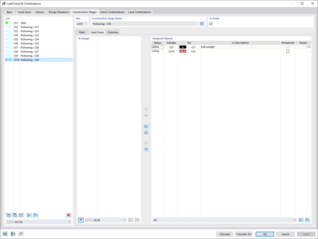
Czy udało Ci się utworzyć całą konstrukcję w programie RFEM? Dobrze, teraz można przypisać poszczególne elementy konstrukcyjne i przypadki obciążeń do odpowiednich etapów budowy. Na każdym etapie budowy można modyfikować na przykład definicje zwolnień prętów i podpór.
Pozwala to na modelowanie zmian konstrukcyjnych, na przykład podczas betonowania dźwigarów mostowych lub osiadania słupów. Przypadki obciążeń utworzone w programie RFEM należy następnie przydzielić do etapów budowy jako obciążenia stałe lub przejściowe.
Czy wiecie, że...? Kombinatoryka umożliwia nakładanie obciążeń stałych i przejściowych w kombinacjach obciążeń. W ten sposób można określić maksymalne siły wewnętrzne dla różnych pozycji dźwigu lub uwzględnić tymczasowe obciążenia montażowe dostępne tylko w jednym etapie budowy.
Jeżeli między idealnym układem a układem, który uległ deformacji z poprzedniego etapu budowy, pojawią się różnice w geometrii, są one porównywane w programie. Następujące po sobie kolejne etapy budowy obliczane są na bazie układu konstrukcyjnego z odkształceniami i obciążeniami wynikającymi z poprzednich etapu budowy. Obliczenia te są nieliniowe.
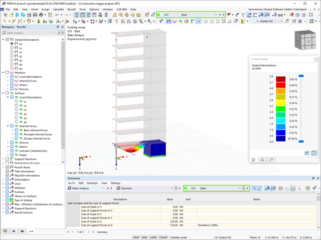
Czy obliczenia zakończyły się pomyślnie? Wyniki poszczególnych etapów budowy można teraz wyświetlać graficznie oraz w tabelach w programie RFEM. Ponadto program RFEM umożliwia uwzględnienie etapów budowy w kombinatoryce i uwzględnienie ich w dalszych obliczeniach.
- 002089
- Ogólne informacje
- Skręcanie skrępowane (7 stopni swobody) RFEM 6
- Skręcanie skrępowane (7 stopni swobody) RSTAB 9
- Uwzględnienie 7 lokalnych kierunków deformacji (ux , uy, uz, φx, φy, φz, ω ) lub 8 sił wewnętrznych (N , Vu, Vv, Mt, pri, Mt, s, Mu, Mv, Mω ) przy obliczaniu elementów prętowych
- Możliwość stosowania w połączeniu z analizą statyczno-wytrzymałościową według teorii II rzędu, i analiza dużych deformacji (można również uwzględnić imperfekcje)
- W połączeniu z rozszerzeniem Analiza stateczności umożliwia definiowanie współczynników obciążenia krytycznego i kształtów drgań dla problemów stateczności, takich jak wyboczenie skrętne i zwichrzenie
- Uwzględnianie blach czołowych i usztywnień poprzecznych jako sprężystości skrępowanej podczas obliczania przekrojów dwuteowych z automatycznym określaniem i wyświetlaniem graficznym sztywności sprężystości deplanacyjnej
- Graficzne przedstawienie deplanacji przekroju prętów w stanie odkształcenia
- Pełna integracja z RFEM i RSTAB
- 002090
- Ogólne informacje
- Skręcanie skrępowane (7 stopni swobody) RFEM 6
- Skręcanie skrępowane (7 stopni swobody) RSTAB 9
Obliczenia skręcania skrępowanego można przeprowadzić dla całego układu. Uwzględniasz zatem dodatkową wartość 7 stopnia swobody w obliczeniach pręta. Sztywności połączonych elementów konstrukcyjnych są uwzględniane automatycznie. Oznacza to, że nie ma potrzeby' definiowania równoważnych sztywności sprężystych ani warunków podparcia dla układu odłączanego.
Następnie można wykorzystać siły wewnętrzne z obliczeń ze skręcaniem skrępowanym w rozszerzeniu do obliczeń. W zależności od materiału i wybranej normy należy uwzględnić bimoment wyboczeniowy i drugorzędny moment skręcający. Typowym zastosowaniem jest analiza stateczności według teorii drugiego rzędu z wykorzystaniem imperfekcji w konstrukcjach stalowych.
Czy wiecie, że...? Zastosowanie nie ogranicza się do przekrojów stalowych cienkościennych. Pozwala to na przykład na przeprowadzenie obliczeń idealnego momentu krytycznego dla belek o przekrojach z drewna litego.