43 Wyniki
Wyświetl wyniki:
Sortuj według:
- 002089
- Ogólne informacje
- Skręcanie skrępowane (7 stopni swobody) RFEM 6
- Skręcanie skrępowane (7 stopni swobody) RSTAB 9
- Uwzględnienie 7 lokalnych kierunków deformacji (ux , uy, uz, φx, φy, φz, ω ) lub 8 sił wewnętrznych (N , Vu, Vv, Mt, pri, Mt, s, Mu, Mv, Mω ) przy obliczaniu elementów prętowych
- Możliwość stosowania w połączeniu z analizą statyczno-wytrzymałościową według teorii II rzędu, i analiza dużych deformacji (można również uwzględnić imperfekcje)
- W połączeniu z rozszerzeniem Analiza stateczności umożliwia definiowanie współczynników obciążenia krytycznego i kształtów drgań dla problemów stateczności, takich jak wyboczenie skrętne i zwichrzenie
- Uwzględnianie blach czołowych i usztywnień poprzecznych jako sprężystości skrępowanej podczas obliczania przekrojów dwuteowych z automatycznym określaniem i wyświetlaniem graficznym sztywności sprężystości deplanacyjnej
- Graficzne przedstawienie deplanacji przekroju prętów w stanie odkształcenia
- Pełna integracja z RFEM i RSTAB

- 002090
- Ogólne informacje
- Skręcanie skrępowane (7 stopni swobody) RFEM 6
- Skręcanie skrępowane (7 stopni swobody) RSTAB 9
Obliczenia skręcania skrępowanego można przeprowadzić dla całego układu. Uwzględniasz zatem dodatkową wartość 7 stopnia swobody w obliczeniach pręta. Sztywności połączonych elementów konstrukcyjnych są uwzględniane automatycznie. Oznacza to, że nie ma potrzeby' definiowania równoważnych sztywności sprężystych ani warunków podparcia dla układu odłączanego.
Następnie można wykorzystać siły wewnętrzne z obliczeń ze skręcaniem skrępowanym w rozszerzeniu do obliczeń. W zależności od materiału i wybranej normy należy uwzględnić bimoment wyboczeniowy i drugorzędny moment skręcający. Typowym zastosowaniem jest analiza stateczności według teorii drugiego rzędu z wykorzystaniem imperfekcji w konstrukcjach stalowych.
Czy wiecie, że...? Zastosowanie nie ogranicza się do przekrojów stalowych cienkościennych. Pozwala to na przykład na przeprowadzenie obliczeń idealnego momentu krytycznego dla belek o przekrojach z drewna litego.
- 002401
- Ogólne informacje
- Skręcanie skrępowane (7 stopni swobody) RFEM 6
- Skręcanie skrępowane (7 stopni swobody) RSTAB 9
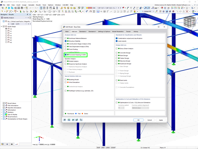
- Funkcję skręcania skrępowanego można aktywować lub dezaktywować w zakładce Rozszerzenia w Danych podstawowych modelu.
- Po aktywowaniu rozszerzenia interfejs użytkownika w programie RFEM zostaje rozszerzony o nowe wpisy w nawigatorze, tabelach i oknach dialogowych.
- Uwzględnianie i wyświetlanie mas kondygnacji
- Lista elementów konstrukcyjnych i ich informacje
- Automatyczne tworzenie przekrojów wynikowych na ścianach usztywniających
- Wyświetlanie wypadkowych przekrojów w kierunku globalnym do wyznaczania sił tnących
- Opcjonalna definicja sztywnej membrany według kondygnacji (modelowanie kondygnacji)
- Typ sztywności Płyta stropowa - tarcza sztywna
- Definiowanie zbiorów stropów,
- na przykład obliczanie płyt jako pozycji 2D w modelu 3D
- Ściany usztywniające: Automatyczne definiowanie prętów wynikowych o dowolnym przekroju
- Wymiarowanie przekrojów prostokątnych z wykorzystaniem rozszerzenia Projektowanie konstrukcji betonowych
- Definicja belek-ścian
- Wymiarowanie możliwe dzięki rozszerzeniu Projektowanie konstrukcji betonowych
- Tabelaryczne przedstawianie oddziaływań kondygnacji, znoszenia międzykondygnacyjnego oraz punktów środkowych masy i sztywności, jak również sił w ścianach usztywniających
- Oddzielne wyświetlanie wyników dla obliczeń stropu i usztywnień
- Opcjonalne pominięcie otworów o określonym rozmiarze
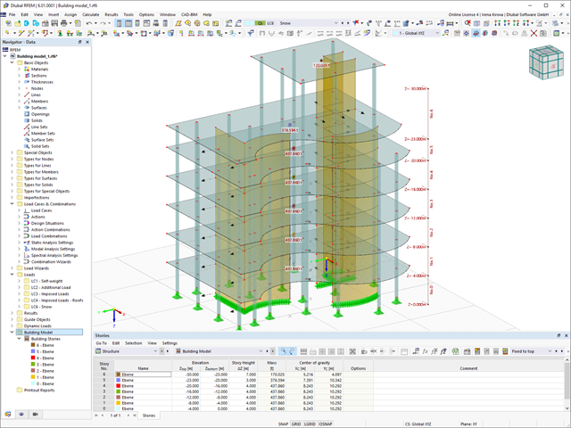
W przypadku modelu budynku dostępne są dwie opcje. Można go utworzyć na początku modelowania konstrukcji lub aktywować później. W modelu budynku można bezpośrednio definiować kondygnacje i modyfikować je.
Podczas manipulowania kondygnacjami można wybrać, czy zostaną zmodyfikowane, czy zachowane, korzystając z różnych opcji.
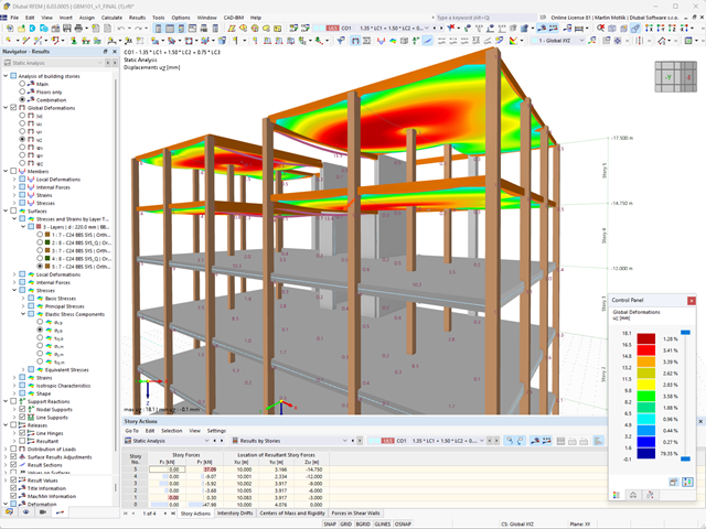
Program RFEM wykonuje część pracy za Ciebie. Na przykład, program automatycznie generuje przekroje wynikowe,'dzięki czemu nie trzeba wykonywać wielu obliczeń.
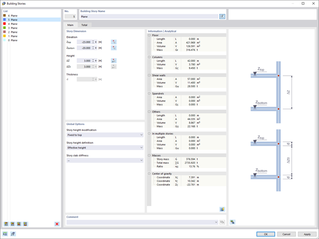
Wyniki można wyświetlić w zwykły sposób za pomocą nawigatora Wyniki. Ponadto w oknie dialogowym rozszerzenia wyświetlane są informacje o poszczególnych kondygnacjach. Dzięki temu zawsze masz dobry przegląd.
_ENG.png?mw=640&hash=1053c9bef400e9f5361c9c3278f76a272fcc4ddf)
Czy aktywowałeś rozszerzenie Analiza historii czasowej (TDA)? Dobrze, teraz można dodawać dane czasowe do przypadków obciążeń. Po zdefiniowaniu początku i końca obciążenia, uwzględniany jest wpływ pełzania na końcu obciążenia. Program umożliwia modelowanie efektów pełzania w konstrukcjach szkieletowych i kratowych wykonanych z betonu zbrojonego.
W tym przypadku obliczenia są przeprowadzane nieliniowo zgodnie z modelem reologicznym (model Kelvina i Maxwella).
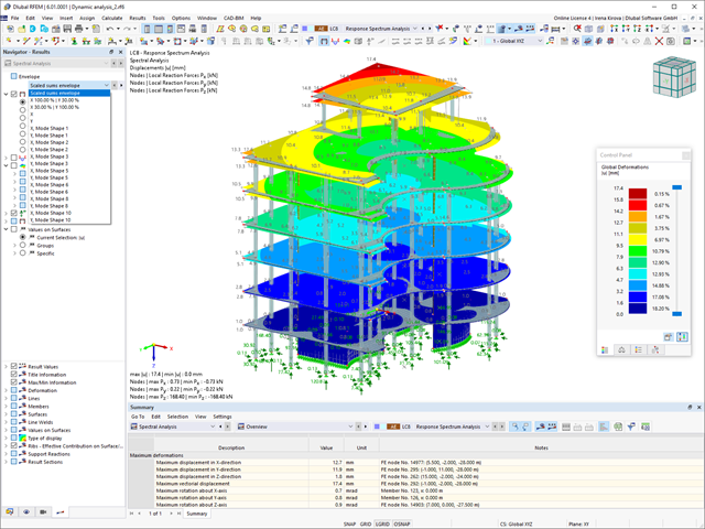
Czy obliczenia zakończyły się pomyślnie? Wyznaczone siły wewnętrzne można teraz wyświetlić w tabelach i grafice, a także uwzględnić w obliczeniach.
Oprogramowanie do analizy statyczno-wytrzymałościowej firmy Dlubal wykonuje wiele pracy za Ciebie. Program sugeruje zgodnie z regułami parametry wejściowe, istotne dla wybranych norm. Ponadto można ręcznie wprowadzić spektra odpowiedzi.
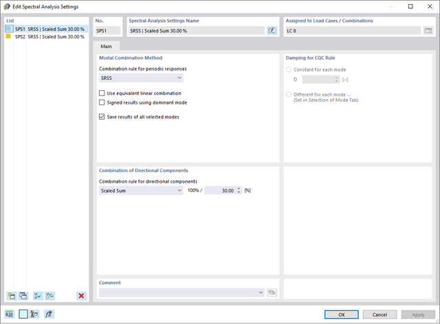
Przypadki obciążeń typu Analiza spektrum odpowiedzi określają kierunek, w którym działają spektra odpowiedzi oraz które wartości własne konstrukcji są istotne dla analizy. W ustawieniach analizy spektralnej można zdefiniować szczegóły dotyczące reguł kombinacji, tłumienia (jeśli ma zastosowanie) i przyspieszenia okresu zerowego (ZPA).
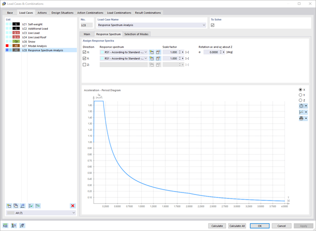
Czy wiecie, że...? Równoważne obciążenia statyczne generowane są oddzielnie dla każdej miarodajnej postaci drgań własnych oraz kierunku wzbudzenia. Obciążenia te są zapisywane w przypadku obciążenia typu Analiza spektrum odpowiedzi, a program RFEM/RSTAB przeprowadza liniową analizę statyczną.
Przypadki obciążeń typu Analiza spektrum odpowiedzi zawierają wygenerowane obciążenia równoważne. Po pierwsze, udziały modalne muszą zostać nałożone na siebie z regułą SRSS lub CQC. W takim przypadku można wykorzystać wyniki podpisane na podstawie dominującego kształtu drgań.
Następnie składowe kierunkowe oddziaływań sejsmicznych są łączone z regułą SRSS lub regułą 100%/30%.

- Definiowanie naprężeń na przykładzie sprężysto-plastycznego modelu materiałowego
- Wymiarowanie murowych konstrukcji tarczowych na ściskanie i ścinanie na modelu budynku lub na pojedynczym modelu
- Automatyczne określanie sztywności przegubu ściana-płyta
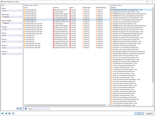
- Obszerna baza danych materiałów o prawie wszystkich kombinacjach kamienia i zapraw dostępnych na rynku austriackim (asortyment jest stale poszerzany, również dla innych krajów)
- Automatyczne określanie wartości materiałów zgodnie z Eurokodem 6 (ÖN EN 1996‑X)
- Możliwość przeprowadzenia analizy pushover
Konstrukcję wprowadza się i modeluje się bezpośrednio w programie RFEM. Model materiałowy muru można połączyć ze wszystkimi popularnymi rozszerzeniami dla programu RFEM. Umożliwia to projektowanie całych modeli budynków w połączeniu z murem.
Program automatycznie określa wszystkie parametry wymagane do obliczeń na podstawie wprowadzonych danych materiału. Następnie generowane są krzywe naprężenie-odkształcenie dla każdego elementu skończonego.
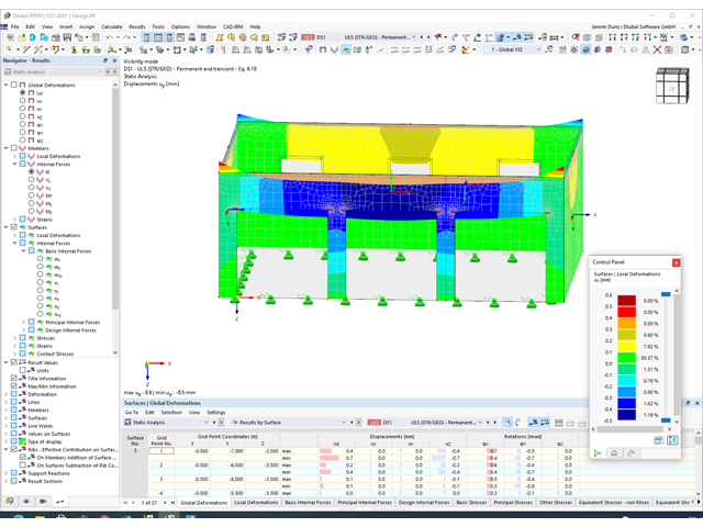
Czy projekt zakończył się sukcesem? Następnie po prostu usiądź i zrelaksuj się. Również tutaj można korzystać z licznych funkcji programu RFEM. Program podaje maksymalne naprężenia powierzchni murowanych, dzięki czemu można szczegółowo wyświetlić wyniki w każdym punkcie siatki ES.
Ponadto można wstawiać przekroje w celu przeprowadzenia szczegółowej analizy poszczególnych obszarów. Na podstawie przedstawionych obszarów uplastycznienia można oszacować zarysowania w murze.
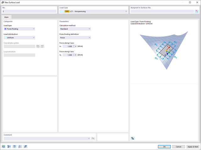
Po aktywowaniu rozszerzenia Form-Finding w Danych ogólnych, efekt znajdowania kształtu jest przypisywany do przypadków obciążeń z kategorią przypadków obciążenia "Sprężenie" w połączeniu z obciążeniami od znajdowania kształtu od pręta, powierzchni i bryły wczytaj katalog. Jest to przypadek obciążenia wstępnego naprężenia. Przekształca się on zatem w analizę znajdowania kształtu dla całego modelu ze zdefiniowanymi w nim wszystkimi elementami prętowymi, powierzchniowymi i bryłowymi. Do znajdowania kształtu odpowiednich elementów prętowych i membranowych dochodzi się w całym modelu za pomocą specjalnych obciążeń w zakresie znajdowania kształtu i regularnych definicji obciążeń. Te obciążenia znajdowania kształtu opisują oczekiwany stan odkształcenia lub siły po wyszukaniu kształtu w elementach. Obciążenia regularne opisują zewnętrzne obciążenie całego układu.
Czy wiesz dokładnie, w jaki sposób przebiega wyszukiwanie kształtu? Po pierwsze, proces znajdowania kształtu przypadków obciążeń z kategorią przypadku obciążenia "Wstępne naprężenie" przesuwa początkową geometrię siatki do optymalnie zrównoważonej pozycji za pomocą iteracyjnych pętli obliczeniowych. W tym celu program wykorzystuje metodę Zaktualizowanej Strategii Odniesienia (URS) opracowaną przez prof. Bletzingera i prof. Ramma. Technologię tę charakteryzują kształty równowagi, które po obliczeniach prawie dokładnie odpowiadają początkowo zadanym warunkom brzegowym (ugięcie, siła i naprężenie wstępne).
Oprócz opisu oczekiwanych sił lub zwisów na elementach, zintegrowane podejście URS umożliwia również uwzględnienie sił regularnych. W całym procesie pozwala to na przykład na opisanie ciężaru własnego lub ciśnienia pneumatycznego za pomocą odpowiednich obciążeń elementów.
Wszystkie te opcje dają rdzeniu obliczeniowemu możliwość obliczania postaci antyklastycznych i synklastycznych, które są w równowadze sił, dla geometrii płaskich lub obrotowo-symetrycznych. Aby możliwe było realistyczne zaimplementowanie obu typów, pojedynczo lub razem w jednym środowisku, w obliczeniach dostępne są dwa sposoby opisania wektorów sił do analizy form-finding:
- Metoda rozciągania - opis znajdowania kształtu wektorów sił w przestrzeni dla geometrii płaskich
- Metoda rzutowania - opis znajdowania kształtu wektorów sił na płaszczyznę rzutowania z ustaleniem położenia poziomego dla geometrii stożkowych
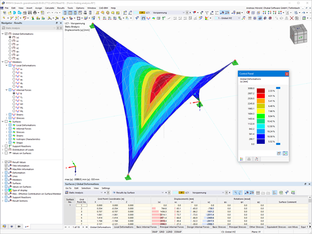
Proces znajdowania kształtu tworzy model konstrukcyjny z aktywnymi siłami w "przypadku obciążenia sprężonego" Ten przypadek obciążenia pokazuje przemieszczenie od początkowego położenia wejściowego do ustalonej geometrii w wynikach deformacji. W wynikach opartych na sile lub naprężeniach (siły wewnętrzne prętów i powierzchni, naprężenia w bryłach, ciśnienia gazu itp.) określany jest stan w celu zachowania znalezionej formy. Do analizy kształtu geometrycznego program oferuje dwuwymiarowy wykres konturowy z przedstawieniem wysokości bezwzględnej i wykresem nachylenia do wizualizacji sytuacji na zboczu.
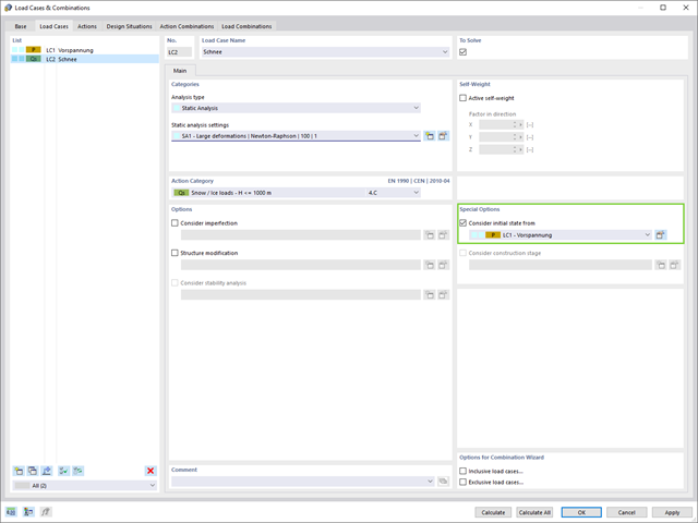
Teraz przeprowadzane są dalsze obliczenia i analiza statyczno-wytrzymałościowa całego modelu. W tym celu program przenosi geometrię zorientowaną na kształt wraz z odkształceniami zależnymi od elementów do uniwersalnego stanu początkowego. Można go teraz używać w przypadkach obciążeń i kombinacjach obciążeń.
W porównaniu z modułem dodatkowym RF-FORM-FINDING (RFEM 5), do modułu Form-Finding dla programu RFEM 6 dodano następujące nowe funkcje:
- Określenie wszystkich warunków brzegowych dotyczących obciążenia dla analizy znajdowania kształtu (form-finding) w pojedynczym przypadku obciążenia
- Przechowywanie wyników analizy znajdowania kształtu jako stanu początkowego z możliwością późniejszego wykorzystania przy dalszej analizie modelu
- Automatyczne przypisywanie stanu początkowego z analizy znajdowania kształtu do wszystkich sytuacji obciążeniowych w sytuacji obliczeniowej za pomocą kreatorów kombinacji
- Dodatkowe geometryczne warunki brzegowe dla prętów (długość elementu nieobciążonego, maksymalny zwis w pionie, zwis w pionie w najniższym punkcie punkcie)
- Dodatkowe warunki brzegowe z uwagi na obciążenie w analizie znajdowania kształtu dla prętów (maksymalna siła w pręcie, minimalna siła w pręcie, rozciągająca składowa pozioma, rozciąganie na i-końcu, rozciąganie na końcu j, minimalne rozciąganie na końcu i, minimalne rozciąganie na końcu j)
- Typ materiału „Tkanina” i „Folia” w bibliotece materiałów
- Równoległe analizy znajdowania kształtu w jednym modelu
- Symulacja kolejnych etapów znajdowania kształtów w połączeniu z rozszerzeniem Analiza etapów konstrukcji (CSA)
- 002165
- Ogólne informacje
- Skręcanie skrępowane (7 stopni swobody) RFEM 6
- Skręcanie skrępowane (7 stopni swobody) RSTAB 9
W porównaniu z modułem dodatkowym RF-/STEEL Warping Torsion (RFEM 5/RSTAB 8) do rozszerzenia Skręcanie skrępowane (7 DOF) dla programu RFEM 6/RSTAB 9 dodano następujące nowe funkcje:
- Pełna integracja ze środowiskiem RFEM 6 i RSTAB 9
- Siódmy stopień swobody jest bezpośrednio uwzględniany w obliczeniach prętów w programie RFEM/RSTAB na całym układzie
- Nie ma już potrzeby definiowania warunków podparcia lub sztywności sprężystej do obliczeń w uproszczonym układzie zastępczym
- Możliwość łączenia z innymi rozszerzeniami, na przykład do obliczania obciążeń krytycznych dla wyboczenia skrętnego i zwichrzenia z analizą stateczności
- Brak ograniczeń dla stalowych przekrojów cienkościennych (możliwe jest również obliczenie momentu krytycznego, na przykład dla belek o masywnych przekrojach drewnianych)
W porównaniu z modułem dodatkowym RF-/DYNAM Pro-Equivalent Loads (RFEM 5/RSTAB 8) do rozszerzenia Analiza spektrum odpowiedzi dla programu RFEM 6/RSTAB 9 dodano następujące nowe funkcje:
- Spektrum odpowiedzi z wielu norm (EN 1998, DIN 4149, IBC 2018 itd.)
- Spektrum odpowiedzi zdefiniowane przez użytkownika lub wygenerowane z akcelerogramów
- Możliwość zadania kierunkowego spektrum odpowiedzi
- Aby zapewnić przejrzystość wyniki są przechowywane łącznie, w jednym przypadku obciążenia, w ramach którego dostępne są różne poziomy wyświetlania
- Wpływ przypadkowych oddziaływań skręcających może być uwzględniany automatycznie
- Automatyczne kombinacje obciążeń sejsmicznych z innymi przypadkami obciążeń, możliwe do wykorzystania w wyjątkowej sytuacji obliczeniowej

Dla każdego przypadku obciążenia można wyświetlić odkształcenia w czasie końcowym.
Wyniki te są również dokumentowane w protokole wydruku programów RFEM i RSTAB. Zawartość protokołu i jego zakres można wybrać specjalnie dla poszczególnych warunków projektowych.