45 Wyniki
Wyświetl wyniki:
Sortuj według:
- Realistyczne odwzorowanie interakcji między budynkiem a gruntem
- Realistyczne odwzorowanie oddziaływania poszczególnych fundamentów na siebie nawzajem
- Biblioteka parametrów gruntowych z możliwością rozszerzania
- Możliwość uwzględniania wielu próbek gruntu z różnych lokalizacji, także poza obrysem budynku
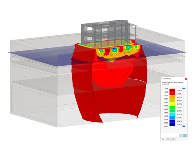
- Określanie osiadań oraz wykresów naprężeń w gruncie oraz ich prezentacja w formie graficznej i tabelarycznej

Wprowadzanie warstw gruntu dla potrzeb zadawania próbek gruntu odbywa się w przejrzystym oknie dialogowym. Odpowiadająca temu prezentacja graficzna zapewnia przejrzystość i ułatwia kontrolę wprowadzanych danych.
Rozszerzalna baza danych ułatwia wybór właściwości materiałowych dla gruntu. Dla realistycznego odwzorowania zachowania się materiału gruntowego można użyć modelu Mohra-Coulomba oraz model gruntu ze wzmocnieniem.
Można zdefiniować dowolną liczbę próbek i warstw gruntu. Grunt jest odwzorowany na podstawie wszystkich wprowadzonych próbek za pomocą brył 3D. Przypisanie do konstrukcji odbywa się za pomocą współrzędnych.
Zachowanie bryły gruntu jest obliczane za pomocą nieliniowej metody iteracyjnej. Obliczone naprężenia i osiadania są wyświetlane graficznie oraz w tabelach.
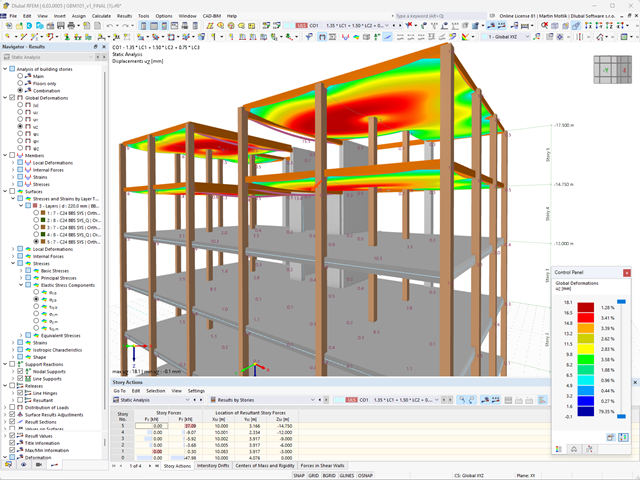
- Uwzględnianie i wyświetlanie mas kondygnacji
- Lista elementów konstrukcyjnych i ich informacje
- Automatyczne tworzenie przekrojów wynikowych na ścianach usztywniających
- Wyświetlanie wypadkowych przekrojów w kierunku globalnym do wyznaczania sił tnących
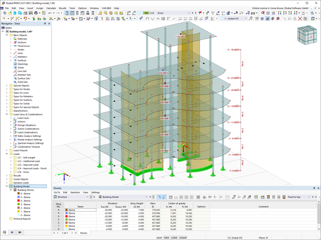
- Opcjonalna definicja sztywnej membrany według kondygnacji (modelowanie kondygnacji)
- Typ sztywności Płyta stropowa - tarcza sztywna
- Definiowanie zbiorów stropów,
- na przykład obliczanie płyt jako pozycji 2D w modelu 3D
- Ściany usztywniające: Automatyczne definiowanie prętów wynikowych o dowolnym przekroju
- Wymiarowanie przekrojów prostokątnych z wykorzystaniem rozszerzenia Projektowanie konstrukcji betonowych
- Definicja belek-ścian
- Wymiarowanie możliwe dzięki rozszerzeniu Projektowanie konstrukcji betonowych
- Tabelaryczne przedstawianie oddziaływań kondygnacji, znoszenia międzykondygnacyjnego oraz punktów środkowych masy i sztywności, jak również sił w ścianach usztywniających
- Oddzielne wyświetlanie wyników dla obliczeń stropu i usztywnień
- Opcjonalne pominięcie otworów o określonym rozmiarze
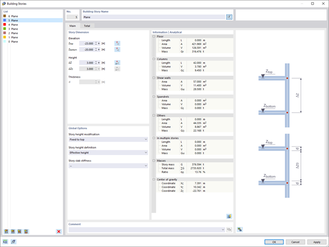
W przypadku modelu budynku dostępne są dwie opcje. Można go utworzyć na początku modelowania konstrukcji lub aktywować później. W modelu budynku można bezpośrednio definiować kondygnacje i modyfikować je.
Podczas manipulowania kondygnacjami można wybrać, czy zostaną zmodyfikowane, czy zachowane, korzystając z różnych opcji.
Program RFEM wykonuje część pracy za Ciebie. Na przykład, program automatycznie generuje przekroje wynikowe,'dzięki czemu nie trzeba wykonywać wielu obliczeń.
Wyniki można wyświetlić w zwykły sposób za pomocą nawigatora Wyniki. Ponadto w oknie dialogowym rozszerzenia wyświetlane są informacje o poszczególnych kondygnacjach. Dzięki temu zawsze masz dobry przegląd.
_ENG.png?mw=640&hash=1053c9bef400e9f5361c9c3278f76a272fcc4ddf)
Czy aktywowałeś rozszerzenie Analiza historii czasowej (TDA)? Dobrze, teraz można dodawać dane czasowe do przypadków obciążeń. Po zdefiniowaniu początku i końca obciążenia, uwzględniany jest wpływ pełzania na końcu obciążenia. Program umożliwia modelowanie efektów pełzania w konstrukcjach szkieletowych i kratowych wykonanych z betonu zbrojonego.
W tym przypadku obliczenia są przeprowadzane nieliniowo zgodnie z modelem reologicznym (model Kelvina i Maxwella).
Czy obliczenia zakończyły się pomyślnie? Wyznaczone siły wewnętrzne można teraz wyświetlić w tabelach i grafice, a także uwzględnić w obliczeniach.
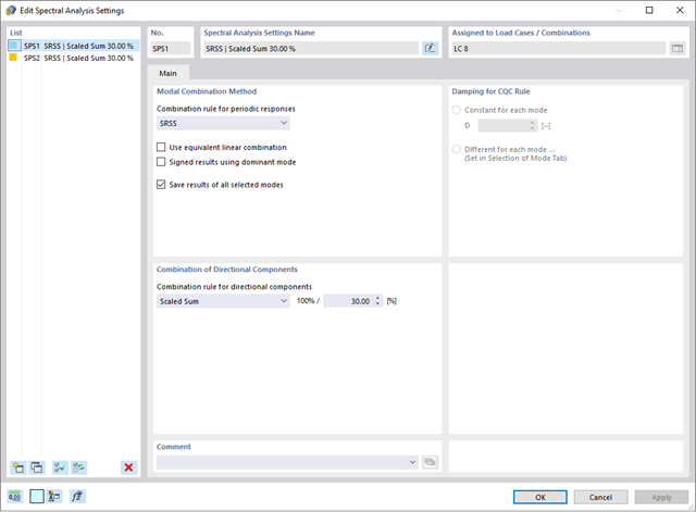
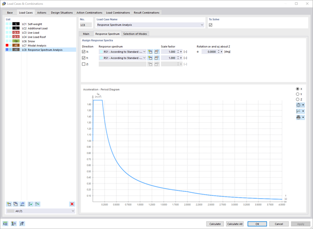
Oprogramowanie do analizy statyczno-wytrzymałościowej firmy Dlubal wykonuje wiele pracy za Ciebie. Program sugeruje zgodnie z regułami parametry wejściowe, istotne dla wybranych norm. Ponadto można ręcznie wprowadzić spektra odpowiedzi.
Przypadki obciążeń typu Analiza spektrum odpowiedzi określają kierunek, w którym działają spektra odpowiedzi oraz które wartości własne konstrukcji są istotne dla analizy. W ustawieniach analizy spektralnej można zdefiniować szczegóły dotyczące reguł kombinacji, tłumienia (jeśli ma zastosowanie) i przyspieszenia okresu zerowego (ZPA).
Czy wiecie, że...? Równoważne obciążenia statyczne generowane są oddzielnie dla każdej miarodajnej postaci drgań własnych oraz kierunku wzbudzenia. Obciążenia te są zapisywane w przypadku obciążenia typu Analiza spektrum odpowiedzi, a program RFEM/RSTAB przeprowadza liniową analizę statyczną.
Przypadki obciążeń typu Analiza spektrum odpowiedzi zawierają wygenerowane obciążenia równoważne. Po pierwsze, udziały modalne muszą zostać nałożone na siebie z regułą SRSS lub CQC. W takim przypadku można wykorzystać wyniki podpisane na podstawie dominującego kształtu drgań.
Następnie składowe kierunkowe oddziaływań sejsmicznych są łączone z regułą SRSS lub regułą 100%/30%.
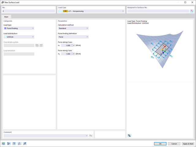
Po aktywowaniu rozszerzenia Form-Finding w Danych ogólnych, efekt znajdowania kształtu jest przypisywany do przypadków obciążeń z kategorią przypadków obciążenia "Sprężenie" w połączeniu z obciążeniami od znajdowania kształtu od pręta, powierzchni i bryły wczytaj katalog. Jest to przypadek obciążenia wstępnego naprężenia. Przekształca się on zatem w analizę znajdowania kształtu dla całego modelu ze zdefiniowanymi w nim wszystkimi elementami prętowymi, powierzchniowymi i bryłowymi. Do znajdowania kształtu odpowiednich elementów prętowych i membranowych dochodzi się w całym modelu za pomocą specjalnych obciążeń w zakresie znajdowania kształtu i regularnych definicji obciążeń. Te obciążenia znajdowania kształtu opisują oczekiwany stan odkształcenia lub siły po wyszukaniu kształtu w elementach. Obciążenia regularne opisują zewnętrzne obciążenie całego układu.
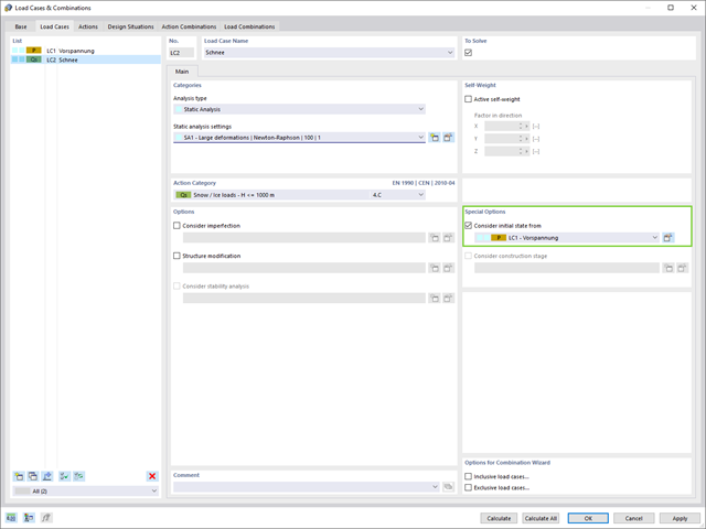
Czy wiesz dokładnie, w jaki sposób przebiega wyszukiwanie kształtu? Po pierwsze, proces znajdowania kształtu przypadków obciążeń z kategorią przypadku obciążenia "Wstępne naprężenie" przesuwa początkową geometrię siatki do optymalnie zrównoważonej pozycji za pomocą iteracyjnych pętli obliczeniowych. W tym celu program wykorzystuje metodę Zaktualizowanej Strategii Odniesienia (URS) opracowaną przez prof. Bletzingera i prof. Ramma. Technologię tę charakteryzują kształty równowagi, które po obliczeniach prawie dokładnie odpowiadają początkowo zadanym warunkom brzegowym (ugięcie, siła i naprężenie wstępne).
Oprócz opisu oczekiwanych sił lub zwisów na elementach, zintegrowane podejście URS umożliwia również uwzględnienie sił regularnych. W całym procesie pozwala to na przykład na opisanie ciężaru własnego lub ciśnienia pneumatycznego za pomocą odpowiednich obciążeń elementów.
Wszystkie te opcje dają rdzeniu obliczeniowemu możliwość obliczania postaci antyklastycznych i synklastycznych, które są w równowadze sił, dla geometrii płaskich lub obrotowo-symetrycznych. Aby możliwe było realistyczne zaimplementowanie obu typów, pojedynczo lub razem w jednym środowisku, w obliczeniach dostępne są dwa sposoby opisania wektorów sił do analizy form-finding:
- Metoda rozciągania - opis znajdowania kształtu wektorów sił w przestrzeni dla geometrii płaskich
- Metoda rzutowania - opis znajdowania kształtu wektorów sił na płaszczyznę rzutowania z ustaleniem położenia poziomego dla geometrii stożkowych
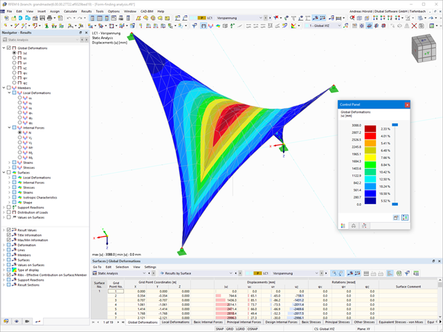
Proces znajdowania kształtu tworzy model konstrukcyjny z aktywnymi siłami w "przypadku obciążenia sprężonego" Ten przypadek obciążenia pokazuje przemieszczenie od początkowego położenia wejściowego do ustalonej geometrii w wynikach deformacji. W wynikach opartych na sile lub naprężeniach (siły wewnętrzne prętów i powierzchni, naprężenia w bryłach, ciśnienia gazu itp.) określany jest stan w celu zachowania znalezionej formy. Do analizy kształtu geometrycznego program oferuje dwuwymiarowy wykres konturowy z przedstawieniem wysokości bezwzględnej i wykresem nachylenia do wizualizacji sytuacji na zboczu.
Teraz przeprowadzane są dalsze obliczenia i analiza statyczno-wytrzymałościowa całego modelu. W tym celu program przenosi geometrię zorientowaną na kształt wraz z odkształceniami zależnymi od elementów do uniwersalnego stanu początkowego. Można go teraz używać w przypadkach obciążeń i kombinacjach obciążeń.
W porównaniu z modułem dodatkowym RF-FORM-FINDING (RFEM 5), do modułu Form-Finding dla programu RFEM 6 dodano następujące nowe funkcje:
- Określenie wszystkich warunków brzegowych dotyczących obciążenia dla analizy znajdowania kształtu (form-finding) w pojedynczym przypadku obciążenia
- Przechowywanie wyników analizy znajdowania kształtu jako stanu początkowego z możliwością późniejszego wykorzystania przy dalszej analizie modelu
- Automatyczne przypisywanie stanu początkowego z analizy znajdowania kształtu do wszystkich sytuacji obciążeniowych w sytuacji obliczeniowej za pomocą kreatorów kombinacji
- Dodatkowe geometryczne warunki brzegowe dla prętów (długość elementu nieobciążonego, maksymalny zwis w pionie, zwis w pionie w najniższym punkcie punkcie)
- Dodatkowe warunki brzegowe z uwagi na obciążenie w analizie znajdowania kształtu dla prętów (maksymalna siła w pręcie, minimalna siła w pręcie, rozciągająca składowa pozioma, rozciąganie na i-końcu, rozciąganie na końcu j, minimalne rozciąganie na końcu i, minimalne rozciąganie na końcu j)
- Typ materiału „Tkanina” i „Folia” w bibliotece materiałów
- Równoległe analizy znajdowania kształtu w jednym modelu
- Symulacja kolejnych etapów znajdowania kształtów w połączeniu z rozszerzeniem Analiza etapów konstrukcji (CSA)
W porównaniu z modułem dodatkowym RF-/DYNAM Pro-Equivalent Loads (RFEM 5/RSTAB 8) do rozszerzenia Analiza spektrum odpowiedzi dla programu RFEM 6/RSTAB 9 dodano następujące nowe funkcje:
- Spektrum odpowiedzi z wielu norm (EN 1998, DIN 4149, IBC 2018 itd.)
- Spektrum odpowiedzi zdefiniowane przez użytkownika lub wygenerowane z akcelerogramów
- Możliwość zadania kierunkowego spektrum odpowiedzi
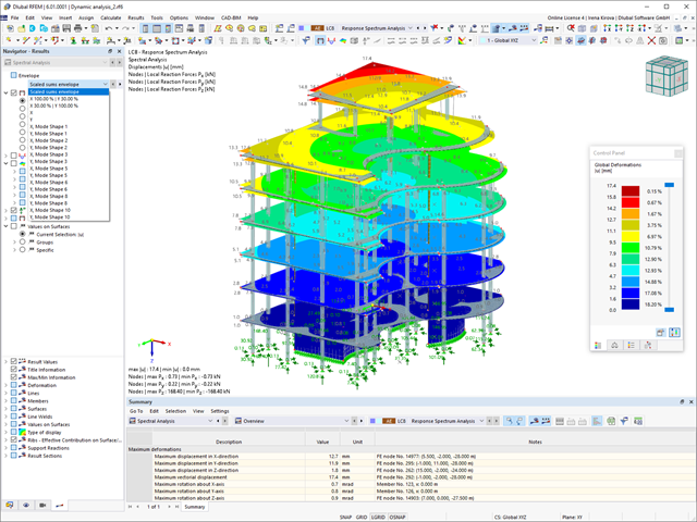
- Aby zapewnić przejrzystość wyniki są przechowywane łącznie, w jednym przypadku obciążenia, w ramach którego dostępne są różne poziomy wyświetlania
- Wpływ przypadkowych oddziaływań skręcających może być uwzględniany automatycznie
- Automatyczne kombinacje obciążeń sejsmicznych z innymi przypadkami obciążeń, możliwe do wykorzystania w wyjątkowej sytuacji obliczeniowej
W porównaniu z modułem dodatkowym RF-SOILIN (RFEM 5) do rozszerzenia Analiza geotechniczna dla programu RFEM 6 dodano następujące nowe funkcje:
- Tworzenie warstwowego gruntu jako modelu 3D z całości zdefiniowanych próbek gruntu
- Symulacja gruntu zgodnie z teorią Mohra-Coulomba
- Graficzne i tabelaryczne przedstawienie naprężeń i odkształceń na dowolnej głębokości gruntu
- Optymalne uwzględnienie interakcji gruntu i konstrukcji na podstawie modelu ogólnego

Dla każdego przypadku obciążenia można wyświetlić odkształcenia w czasie końcowym.
Wyniki te są również dokumentowane w protokole wydruku programów RFEM i RSTAB. Zawartość protokołu i jego zakres można wybrać specjalnie dla poszczególnych warunków projektowych.
Obawiasz się, że Twój projekt skończy się cyfrową wieżą Babel? Rozszerzenie Model budynku dla RFEM wspomaga pracę nad wielokondygnacyjnym projektem budowlanym. Tutaj możesz definiować i manipulować budynkiem za pomocą kondygnacji. Kondygnacje można później dostosować na wiele sposobów, a także wybrać sztywność płyty. Informacje na temat kondygnacji i całego modelu (środek ciężkości, środek sztywności) są wyświetlane w tabelach i na grafice.
Dzięki rozszerzeniu Analiza historii czasowej (TDA) można uwzględnić zmienne w czasie zachowanie materiału w przypadku prętów i powierzchni. Długotrwałe efekty, takie jak pełzanie, skurcz i starzenie, mogą wpływać na rozkład sił wewnętrznych, w zależności od konstrukcji. Darauf bereiten Sie sich mit diesem Add-On optimal vor.
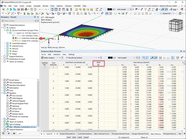
Wyniki naprężeń i odkształceń według powierzchni można wyświetlić w tabeli wyników powierzchni zgodnie z grubością warstwy.
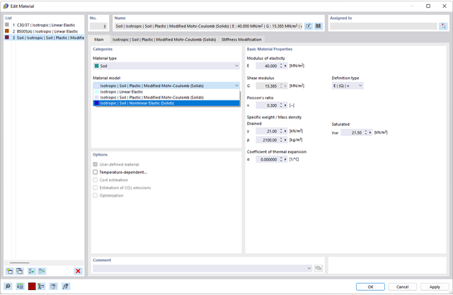
Czy chcesz modelować i analizować zachowanie bryły gruntowej? Aby to zapewnić, w programie RFEM zaimplementowano odpowiednie modele materiałowe.
Można użyć zmodyfikowanego modelu Mohra-Coulomba z liniowo-sprężystym modelem idealnie plastycznym lub nieliniowo sprężystym modelem z edometryczną relacją naprężenie-odkształcenie. Kryterium graniczne, które opisuje przejście od obszaru sprężystości do obszaru płynięcia plastycznego, jest zdefiniowane według Mohra-Coulomba.