63 Wyniki
Wyświetl wyniki:
Sortuj według:
- Automatyczne uwzględnianie masy własnej od ciężaru konstrukcji
- Możliwy bezpośredni import mas z przypadków obciążeń lub kombinacji
- Opcjonalne definiowanie mas dodatkowych (masy węzłowe, liniowe lub powierzchniowe oraz masy wynikające z bezwładności) bezpośrednio w przypadkach obciążeń
- Opcjonalne pominięcie mas (na przykład masy fundamentów)
- Kombinacje mas w różnych przypadkach i kombinacjach obciążeń
- Predefiniowane współczynniki kombinacji wg różnych norm (EC 8, SIA 261, ASCE 7, ...)
- Opcjonalny import stanów początkowych (np. w celu uwzględnienia naprężenia wstępnego i imperfekcji)
- modyfikacja konstrukcji
- Uwzględnianie uszkodzenia w podporach lub prętach/powierzchniach/bryłach
- Możliwość zadania kilku analiz modalnych (np. w celu analizy różnych mas lub modyfikacji sztywności)
- Wybór typu macierzy mas (macierz diagonalna, macierz spójna, macierz jednostkowa) oraz wskazanych przez użytkownika stopni swobody (translacyjne i rotacyjne)
- Metody określania liczby postaci drgań własnych (liczba zdefiniowana przez użytkownika, liczba określana automatycznie - w celu osiągnięcia zadanych efektywnych współczynników masy modalnej, liczba określana automatycznie - w celu osiągnięcia maksymalnej częstotliwości drgań własnych - dostępne tylko w programie RSTAB)
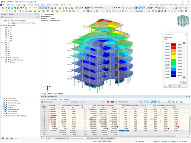
- Określanie postaci drgań i mas w węzłach siatki MES
- Wyniki w postaci wartości własnych, częstości kątowych, częstotliwości drgań własnych i okresu drgań własnych
- Wyniki w postaci mas modalnych, efektywnych mas modalnych, współczynników masy modalnej i współczynników udziału masy
- Tabelaryczne i graficzne przedstawienie mas w punktach siatki MES
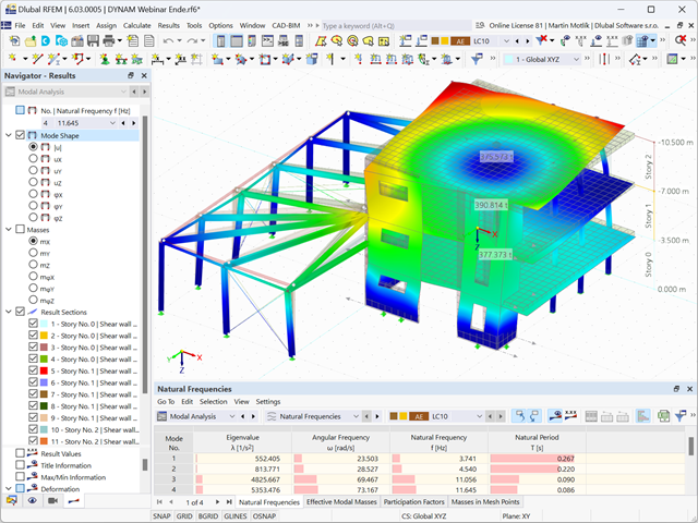
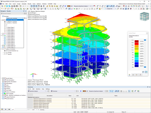
- Wizualizacja i animacja postaci drgań własnych
- Różne opcje skalowania postaci drgań własnych
- Dokumentacja wyników numerycznych i graficznych w raporcie
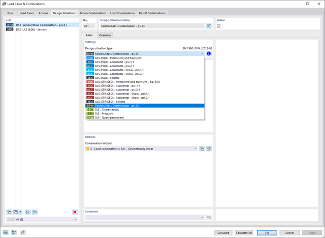
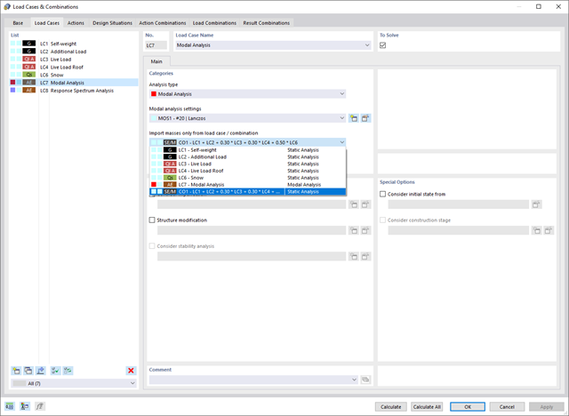
W ustawieniach analizy modalnej należy wprowadzić wszystkie dane, które są niezbędne do określenia częstotliwości drgań własnych. Są to na przykład kształty mas i solwery wartości własnych.
Rozszerzenie Analiza modalna określa najniższe wartości częstości drgań własnych konstrukcji. Liczbę wartości własnych można dostosować lub określić automatycznie. Należy zatem osiągnąć efektywne współczynniki masy modalnej lub maksymalne częstotliwości drgań własnych. Masy są importowane bezpośrednio z przypadków obciążeń i kombinacji obciążeń. W takim przypadku istnieje możliwość uwzględnienia masy całkowitej, składowych obciążenia w globalnym kierunku Z lub tylko składowej obciążenia w kierunku siły ciężkości.
Dodatkowe masy w węzłach, liniach, prętach lub powierzchniach można zdefiniować ręcznie. Ponadto można wpływać na macierz sztywności poprzez import sił osiowych lub modyfikacji sztywności z przypadku obciążenia lub kombinacji obciążeń.
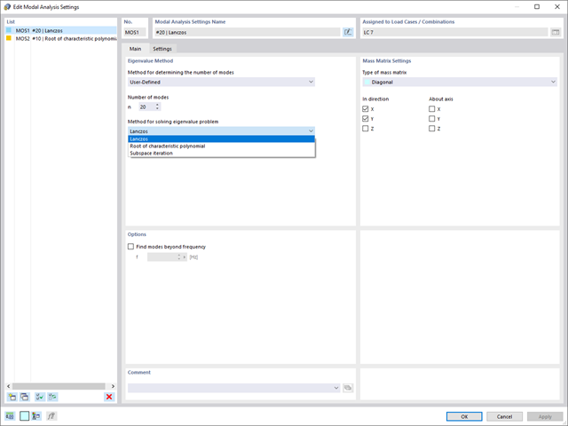
W programie RFEM dostępne są trzy wydajne solwery wartości własnych:
- pierwiastek wielomianu charakterystycznego
- Metoda Lanchosa
- iteracja podprzestrzeni
Z kolei program RSTAB oferuje dwa solwery wartości własnych:
- iteracja podprzestrzeni
- Metoda Powera z przesuniętą odwrotnością
Wybór solwera wartości własnych zależy przede wszystkim od rozmiaru modelu.
Zaraz po zakończeniu obliczeń wyświetlane są wartości własne, częstotliwości drgań własnych i okresy. Okna z tymi wynikami zintegrowane są z programem głównym RFEM/RSTAB. W tabelach można znaleźć wszystkie kształty drgań konstrukcji, a także można je wyświetlić graficznie i animować.
Wszystkie tabele wyników i grafiki stanowią część raportu programu RFEM/RSTAB. Zapewnia to przejrzystą dokumentację obliczeń. Tabele można również eksportować do programu MS Excel.
_ENG.png?mw=640&hash=1053c9bef400e9f5361c9c3278f76a272fcc4ddf)
Czy aktywowałeś rozszerzenie Analiza historii czasowej (TDA)? Dobrze, teraz można dodawać dane czasowe do przypadków obciążeń. Po zdefiniowaniu początku i końca obciążenia, uwzględniany jest wpływ pełzania na końcu obciążenia. Program umożliwia modelowanie efektów pełzania w konstrukcjach szkieletowych i kratowych wykonanych z betonu zbrojonego.
W tym przypadku obliczenia są przeprowadzane nieliniowo zgodnie z modelem reologicznym (model Kelvina i Maxwella).
Czy obliczenia zakończyły się pomyślnie? Wyznaczone siły wewnętrzne można teraz wyświetlić w tabelach i grafice, a także uwzględnić w obliczeniach.
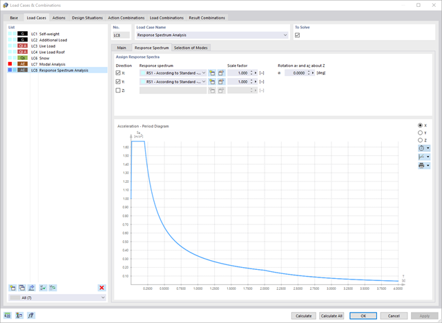
Oprogramowanie do analizy statyczno-wytrzymałościowej firmy Dlubal wykonuje wiele pracy za Ciebie. Program sugeruje zgodnie z regułami parametry wejściowe, istotne dla wybranych norm. Ponadto można ręcznie wprowadzić spektra odpowiedzi.
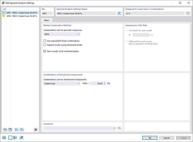
Przypadki obciążeń typu Analiza spektrum odpowiedzi określają kierunek, w którym działają spektra odpowiedzi oraz które wartości własne konstrukcji są istotne dla analizy. W ustawieniach analizy spektralnej można zdefiniować szczegóły dotyczące reguł kombinacji, tłumienia (jeśli ma zastosowanie) i przyspieszenia okresu zerowego (ZPA).
Czy wiecie, że...? Równoważne obciążenia statyczne generowane są oddzielnie dla każdej miarodajnej postaci drgań własnych oraz kierunku wzbudzenia. Obciążenia te są zapisywane w przypadku obciążenia typu Analiza spektrum odpowiedzi, a program RFEM/RSTAB przeprowadza liniową analizę statyczną.
Przypadki obciążeń typu Analiza spektrum odpowiedzi zawierają wygenerowane obciążenia równoważne. Po pierwsze, udziały modalne muszą zostać nałożone na siebie z regułą SRSS lub CQC. W takim przypadku można wykorzystać wyniki podpisane na podstawie dominującego kształtu drgań.
Następnie składowe kierunkowe oddziaływań sejsmicznych są łączone z regułą SRSS lub regułą 100%/30%.

- 002108
- Ogólne informacje
- Optymalizacja i koszty | Szacowanie emisji CO2 RFEM 6
- Optymalizacja i koszty | Szacowanie emisji CO2 RSTAB 9
- Technologia sztucznej inteligencji (AI): Optymalizacja roju cząstek (PSO)
- Optymalizacja konstrukcji ze względu na minimalny ciężar lub deformację
- Możliwość zastosowania dowolnej liczby parametrów optymalizacyjnych
- Określanie zakresów zmiennych
- Optymalizacja przekrojów i materiałów
- Typy definicji parametrów
- Optymalizacja | Rosnąco, czyli optymalizacja | Malejąca
- Zastosowanie parametrycznych modeli i bloków
- Parametryzacja bloków w języku JavaScript na podstawie kodu
- Optymalizacja z uwzględnieniem wyników obliczeń
- Tabelaryczne przedstawienie najlepszych mutacji modelu
- Wyświetlanie w czasie rzeczywistym mutacji modelu w procesie optymalizacji
- Kalkulacja kosztów modelu dzięki zadanym cenom jednostkowym
- Określanie potencjału tworzenia efektu cieplarnianego (GWP-global warming potential) na etapie tworzenia modelu poprzez szacowanie równoważnej emisji CO2
- Określanie jednostkowych wskaźników zależnych od masy, objętości i powierzchni (cena i emisja CO2)

- 002109
- Ogólne informacje
- Optymalizacja i koszty | Szacowanie emisji CO2 RFEM 6
- Optymalizacja i koszty | Szacowanie emisji CO2 RSTAB 9
Masz pytania dotyczące programu? Optymalizacja konstrukcji w programach RFEM i RSTAB jest uzupełnieniem parametrycznego wprowadzania danych. Jest to proces równoległy, niezależny od rzeczywistych obliczeń modelu wraz ze wszystkimi jego zwykłymi definicjami obliczeń i obliczeń. Rozszerzenie zakłada, że model lub blok jest zbudowany w kontekście parametrycznym i jest kontrolowany przez globalne parametry kontrolne typu "optymalizacja". Dlatego te parametry kontrolne mają dolną i górną granicę oraz wielkość kroku w celu ograniczenia zakresu optymalizacji. Aby znaleźć optymalne wartości parametrów kontrolnych, należy określić kryterium optymalizacji (na przykład minimalny ciężar) przy wyborze metody optymalizacji (na przykład optymalizacja roju cząstek).
Oszacowanie kosztów i emisji CO2 można znaleźć już w definicjach materiałów. Obie opcje można aktywować osobno w każdej definicji materiału. Oszacowanie oparte jest na koszcie jednostkowym lub jednostkowej wartości emisji dla prętów, powierzchni oraz brył. W tym przypadku można wybrać, czy jednostki mają zostać podane według masy, objętości czy powierzchni.

- 002110
- Ogólne informacje
- Optymalizacja i koszty | Szacowanie emisji CO2 RFEM 6
- Optymalizacja i koszty | Szacowanie emisji CO2 RSTAB 9
Istnieją dwie metody optymalizacji, dzięki którym można znaleźć optymalne wartości parametrów według kryterium ciężaru lub odkształcenia.
Najbardziej wydajną metodą o najkrótszym czasie obliczeń jest optymalizacja roju cząstek zbliżona do naturalnej (PSO). Czy słyszałeś lub czytałeś o tym? Ta technologia sztucznej inteligencji (AI) ma silną analogię do zachowania stad zwierząt szukających miejsca odpoczynku. W takich rojach można znaleźć wiele osób (por. rozwiązanie optymalizacyjne - na przykład waga), które lubią przebywać w grupie i podążać za ruchem grupy. Załóżmy, że każdy pręt roju musi zostać poddany spoczynkowi w optymalnym miejscu (por. najlepsze rozwiązanie - na przykład najniższa waga). Potrzeba ta wzrasta wraz ze zbliżaniem się do miejsca odpoczynku. Na zachowanie roju mają zatem wpływ również właściwości przestrzeni (por. wykres wyników).
Dlaczego wycieczka do biologii? Po prostu - proces PSO w RFEM lub RSTAB przebiega w podobny sposób. Proces obliczeń rozpoczyna się od wyniku optymalizacji poprzez losowe przypisanie parametrów, które mają zostać zoptymalizowane. Wielokrotnie określa nowe wyniki optymalizacji ze zróżnicowanymi wartościami parametrów, które opierają się na doświadczeniach z wcześniej przeprowadzonych mutacji modelu. Proces jest kontynuowany do momentu osiągnięcia określonej liczby możliwych mutacji modelu.
Jako alternatywa dla tej metody program oferuje również metodę przetwarzania wsadowego. Metoda ta ma na celu sprawdzenie wszystkich możliwych mutacji modelu poprzez losowe określanie wartości parametrów optymalizacji, aż do osiągnięcia określonej liczby możliwych mutacji modelu.
Po obliczeniu mutacji modelu obydwa warianty sprawdzają również odpowiednie aktywowane wyniki obliczeń rozszerzeń. Ponadto zapisuje on wariant z odpowiednim wynikiem optymalizacji i przypisaniem wartości parametrów optymalizacji, jeżeli wykorzystanie jest < 1.
Na podstawie odpowiednich sum poszczególnych materiałów można określić szacunkowe koszty całkowite i emisję. Na sumę materiałów składają się zależne od ciężaru, objętości i powierzchnie elementów prętowych, powierzchniowych i bryłowych.

- 002161
- Ogólne informacje
- Optymalizacja i koszty | Szacowanie emisji CO2 RFEM 6
- Optymalizacja i koszty | Szacowanie emisji CO2 RSTAB 9
Obie metody optymalizacji mają jedną wspólną cechę. Na końcu procesu wyświetlają listę wariacji modelu na podstawie przechowywanych danych. Można tu znaleźć szczegóły na temat wyniku decydującego dla optymalizacji i odpowiadające mu wartości parametrów. Lista jest zorganizowana w porządku malejącym. Zakładane najlepsze rozwiązanie znajduje się na górze. W takim przypadku wynik optymalizacji wraz z wyznaczoną wartością jest najbardziej zbliżony do kryterium optymalizacji. Wszystkie dodatkowe wyniki pokazują wykorzystanie < 1. Ponadto, po zakończeniu analizy, program dostosuje wartości na globalnej liście parametrów, aby odpowiadały tym dla optymalnego rozwiązania.
W oknach dialogowych materiałów znajdują się dodatkowe zakładki "Oszacowanie kosztów" i "Oszacowanie emisji CO2". Tutaj wyświetlane są indywidualne szacunkowe sumy przydzielonych prętów, powierzchni i objętości na jednostkę masy, objętości i powierzchni. Dodatkowo zakładki te podają całkowity koszt i emisję wszystkich przydzielonych do konstrukcji materiałów. Zapewnia to dobry przegląd projektu.
W porównaniu z modułem dodatkowym RF-/DYNAM Pro-Natural Vibrations (RFEM 5/RSTAB 8) do rozszerzenia Analiza modalna dla programu RFEM 6/RSTAB 9 dodano następujące nowe funkcje:
- Predefiniowane współczynniki kombinacji dla różnych norm (EC 8, ASCE itp.)
- Opcjonalne pominięcie mas (na przykład masy fundamentów)
- Metody określania liczby postaci drgań własnych (liczba zdefiniowana przez użytkownika, liczba określana automatycznie - w celu osiągnięcia zadanych efektywnych współczynników masy modalnej, liczba określana automatycznie - w celu osiągnięcia maksymalnej częstotliwości drgań własnych)
- Wyniki w postaci mas modalnych, efektywnych mas modalnych, współczynników masy modalnej i współczynników udziału masy
- Tabelaryczne i graficzne przedstawienie mas w punktach siatki MES
- Różne opcje skalowania postaci drgań własnych w nawigatorze wyników
W porównaniu z modułem dodatkowym RF-/DYNAM Pro-Equivalent Loads (RFEM 5/RSTAB 8) do rozszerzenia Analiza spektrum odpowiedzi dla programu RFEM 6/RSTAB 9 dodano następujące nowe funkcje:
- Spektrum odpowiedzi z wielu norm (EN 1998, DIN 4149, IBC 2018 itd.)
- Spektrum odpowiedzi zdefiniowane przez użytkownika lub wygenerowane z akcelerogramów
- Możliwość zadania kierunkowego spektrum odpowiedzi
- Aby zapewnić przejrzystość wyniki są przechowywane łącznie, w jednym przypadku obciążenia, w ramach którego dostępne są różne poziomy wyświetlania
- Wpływ przypadkowych oddziaływań skręcających może być uwzględniany automatycznie
- Automatyczne kombinacje obciążeń sejsmicznych z innymi przypadkami obciążeń, możliwe do wykorzystania w wyjątkowej sytuacji obliczeniowej
- 002172
- Ogólne informacje
- Projektowanie konstrukcji drewnianych RFEM 6
- Projektowanie konstrukcji drewnianych RSTAB 9
W porównaniu z modułem dodatkowym RF-/TIMBER Pro (RFEM 5/RSTAB 8) do rozszerzenia Projektowanie konstrukcji drewnianych dla programu RFEM 6/RSTAB 9 dodano następujące nowe funkcje:
- Oprócz Eurokodu 5, uwzględnione zostały inne międzynarodowe normy (SIA 265, ANSI/AWC NDS, CSA O86, GB 50005)
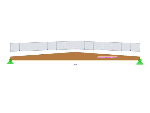
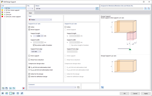
- Obliczanie ściskania prostopadle do włókien (ciśnienie na podporze)
- Wprowadzenie solwera wartości własnych do wyznaczania momentu krytycznego dla wyboczenia skrętnego (tylko EC 5)
- Definicja różnych długości efektywnych do obliczeń w normalnej temperaturze i odporności ogniowej
- Ocena naprężeń poprzez naprężenia jednostkowe (MES)
- Zoptymalizowane analizy stateczności dla prętów o zbieżnym przekroju
- Ujednolicenie materiałów dla wszystkich załączników krajowych (w bibliotece materiałów dostępna jest teraz tylko jedna norma „EN”)
- Wyświetlanie osłabień przekrojów bezpośrednio w renderingu
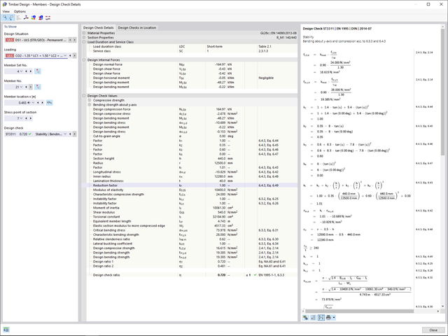
- Wyświetlanie odpowiednich wzorów użytych do sprawdzania warunków nośności (w tym odniesienie do zastosowanego równania z normy)

Dla każdego przypadku obciążenia można wyświetlić odkształcenia w czasie końcowym.
Wyniki te są również dokumentowane w protokole wydruku programów RFEM i RSTAB. Zawartość protokołu i jego zakres można wybrać specjalnie dla poszczególnych warunków projektowych.

- 002232
- Ogólne informacje
- Optymalizacja i koszty | Szacowanie emisji CO2 RFEM 6
- Optymalizacja i koszty | Szacowanie emisji CO2 RSTAB 9
Możesz być pewien, że koszty są ważnym czynnikiem w planowaniu konstrukcyjnym każdego projektu. Należy również przestrzegać przepisów dotyczących szacowania emisji. Dwuczęściowe rozszerzenie Optymalizacja i koszty/Szacowanie emisji CO2 ułatwia odnalezienie się w gąszczu norm i opcji. Wykorzystuje technologię sztucznej inteligencji (AI) optymalizacji rojem cząstek (PSO) w celu znalezienia odpowiednich parametrów dla sparametryzowanych modeli i bloków, które zagwarantują zgodność ze zwykłymi kryteriami optymalizacji. Ponadto, rozszerzenie oszacowuje koszty modelu lub emisję CO2 poprzez określenie kosztów jednostkowych lub emisji jednostkowej dla materiałów zdefiniowanych w modelu konstrukcyjnym. Dzięki temu rozszerzeniu jesteś po bezpiecznej stronie.
Dzięki rozszerzeniu Analiza historii czasowej (TDA) można uwzględnić zmienne w czasie zachowanie materiału w przypadku prętów i powierzchni. Długotrwałe efekty, takie jak pełzanie, skurcz i starzenie, mogą wpływać na rozkład sił wewnętrznych, w zależności od konstrukcji. Darauf bereiten Sie sich mit diesem Add-On optimal vor.
- 002369
- Ogólne informacje
- Projektowanie konstrukcji drewnianych RFEM 6
- Projektowanie konstrukcji drewnianych RSTAB 9
- Obliczanie ugięć i porównanie z normatywnymi lub ręcznie dostosowanymi wartościami granicznymi
- Uwzględnienie wygięcia wstępnego w analizie ugięcia
- W zależności od typu sytuacji obliczeniowej możliwe są różne wartości graniczne
- Ręczne dostosowywanie długości odniesienia i segmentacji według kierunku
- Obliczanie ugięć w odniesieniu do konstrukcji początkowej lub do konstrukcji odkształconej
- Automatyczne uwzględnienie odkształceń zależnych od czasu poprzez zwiększenie obciążenia o współczynnik pełzania (może być również zdefiniowany przez użytkownika po stronie sztywności)
- Uproszczone obliczenia drgań
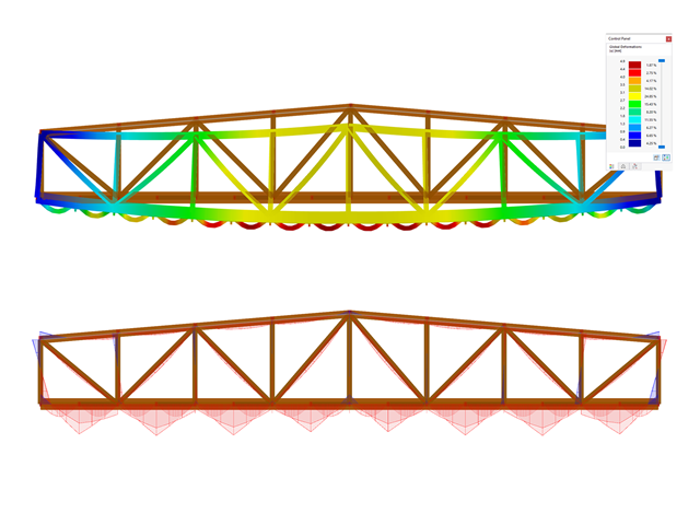
- Graficzne wyświetlanie wyników zintegrowane z RFEM/RSTAB; na przykład stopień wykorzystania wartości granicznej, odkształcenie lub ugięcie
- Pełna integracja wyników z protokołem wydruku programu RFEM/RSTAB
- 002370
- Ogólne informacje
- Projektowanie konstrukcji drewnianych RFEM 6
- Projektowanie konstrukcji drewnianych RSTAB 9
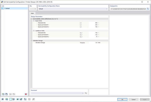
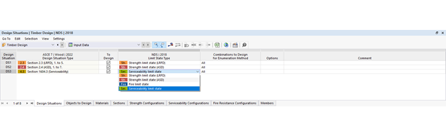
Za wygenerowanie i obliczenie kombinacji obciążeń i wyników wymaganych dla stanu granicznego użytkowalności odpowiada program RFEM/RSTAB. W rozszerzeniu Projektowanie konstrukcji drewnianych można wybrać sytuacje obliczeniowe do analizy ugięć. Obliczone wartości odkształceń są następnie określane w każdym miejscu pręta, w zależności od określonego wygięcia wstępnego i układu odniesienia, a następnie porównywane z wartościami granicznymi.
Wartość graniczną deformacji można określić indywidualnie dla każdego elementu konstrukcyjnego w Konfiguracja stanu granicznego użytkowalności. W takim przypadku maksymalne odkształcenie nie powinno przekraczać dopuszczalnej wartości granicznej, zależnej od długości odniesienia. Podczas definiowania podpór obliczeniowych można podzielić komponenty na segmenty. Umożliwia to automatyczne określenie odpowiedniej długości odniesienia dla każdego kierunku obliczeń.
Na podstawie położenia przypisanych podpór obliczeniowych program automatycznie określa różnicę między belkami a wspornikami. W ten sposób można mieć pewność, że wartość graniczna zostanie odpowiednio określona.
- 002371
- Ogólne informacje
- Projektowanie konstrukcji drewnianych RFEM 6
- Projektowanie konstrukcji drewnianych RSTAB 9
Obliczenia stanu granicznego użytkowalności są w pełni zintegrowane z tabelami wyników w rozszerzeniu Projektowanie konstrukcji drewnianych. Aby sprawdzić wyniki obliczeń, można otworzyć program i wyświetlić wyniki ze wszystkimi szczegółami w każdym miejscu obliczanych prętów. Ponadto dostępne są grafiki z wykresami wyników i stopni wykorzystania.
Cechą szczególną jest to, że Wszystkie tabele wyników i grafiki można zintegrować z globalnym protokołem wydruku programu RFEM/RSTAB jako część wyników wymiarowania drewna. Odkształcenia całej konstrukcji można również wyświetlać i dokumentować w ramach funkcji programu RFEM/RSTAB. Ta funkcja jest niezależna od rozszerzenia.

- 002133
- Ogólne informacje
- Projektowanie konstrukcji drewnianych RFEM 6
- Projektowanie konstrukcji drewnianych RSTAB 9
- Szeroki wybór przekrojów, takich jak przekroje prostokątne, kwadratowe, teowe, okrągłe, złożone, nieregularne przekroje parametryczne i wiele innych (przydatność do obliczeń zależy od wybranej normy)
- Wymiarowanie drewna klejonego krzyżowo (CLT)
- Wymiarowanie materiałów drewnopochodnych i drewna klejonego warstwowo zgodnie z EC 5
- Wymiarowanie prętów o zmiennym przekroju (metoda zgodna z normą)
- Możliwe jest dostosowanie istotnych współczynników obliczeniowych i parametrów normowych
- Elastyczność dzięki szczegółowym opcjom ustawień dla podstawy i zakresu obliczeń
- Szybkie i przejrzyste wyświetlanie wyników dla globalnej oceny ich rozkładu na konstrukcji po zakończeniu obliczeń
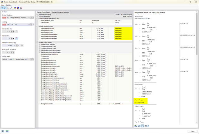
- Szczegółowe wyniki obliczeń i niezbędne wzory (jasna i łatwa do zweryfikowania ścieżka wyników)
- Przejrzyste zestawienie wyników w formie numerycznej w stosownych oknach oraz możliwość ich graficznego przedstawienia na konstrukcji
- Integracja wyników z protokołem wydruku programu RFEM/RSTAB
- 002134
- Ogólne informacje
- Projektowanie konstrukcji drewnianych RFEM 6
- Projektowanie konstrukcji drewnianych RSTAB 9
- Wymiarowanie elementów rozciąganych, ściskanych, zginanych, ścinanych, skręcanych i poddanych połączonemu działaniu tych sił wewnętrznych
- Uwzględnienie podcięcia
- Obliczanie ściskania prostopadle do włókien na podporach końcowych i pośrednich z (EC 5) i bez elementów wzmacniających (śruby z pełnym gwintem)
- Opcjonalna redukcja siły tnącej na podporze
- Wymiarowanie prętów zakrzywionych i zbieżnych
- Uwzględnianie wyższych wytrzymałości dla podobnych elementów, które znajdują się blisko siebie (współczynnik ksys wg EN 1995-1-1, 6.6(1)-(3))
- Możliwość zwiększenia nośności na ścinanie dla drewna iglastego zgodnie z DIN EN 1995‑1‑1:NA NDP do 6.1.7(2)
- 002135
- Obliczenia
- Projektowanie konstrukcji drewnianych RFEM 6
- Projektowanie konstrukcji drewnianych RSTAB 9
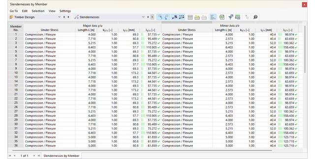
- Analiza stateczności dla wyboczenia giętnego, wyboczenia skrętnego i wyboczenia giętno-skrętnego przy ściskaniu
- Import długości efektywnych z obliczeń przy użyciu rozszerzenia Stateczność konstrukcji
- Graficzne wprowadzanie i kontrola zdefiniowanych podpór węzłowych oraz długości efektywnych w celu analizy stateczności
- Określanie długości zastępczych prętów o zbieżnym przekroju
- Uwzględnienie położenia stężenia zwichrzenia
- Analiza zwichrzenia elementów poddanych obciążeniu momentem
- W zależności od normy istnieje wybór między wprowadzaniem wartości Mcr przez użytkownika, metodą analityczną z normy lub wykorzystaniem wewnętrznego solwera wartości własnych
- Uwzględnienie panelu usztywniającego i ograniczenia obrotu podczas korzystania z solwera wartości własnych
- Graficzne przedstawienie postaci własnej w przypadku zastosowania solwera wartości własnych
- Analiza stateczności elementów konstrukcyjnych ze ściskaniem i naprężeniem zginającym, w zależności od normy obliczeniowej
- Przejrzyste obliczenia wszystkich niezbędnych współczynników, takich jak współczynniki uwzględniające rozkładu momentów lub współczynniki interakcji
- Alternatywne uwzględnienie wszystkich wpływów dla analizy stateczności podczas określania sił wewnętrznych w programie RFEM/RSTAB (analiza drugiego rzędu, imperfekcje, redukcja sztywności, ewentualnie w połączeniu z rozszerzeniem Skręcanie skrępowane (7 stopni swobody))
- 002372
- Ogólne informacje
- Projektowanie konstrukcji drewnianych RFEM 6
- Projektowanie konstrukcji drewnianych RSTAB 9
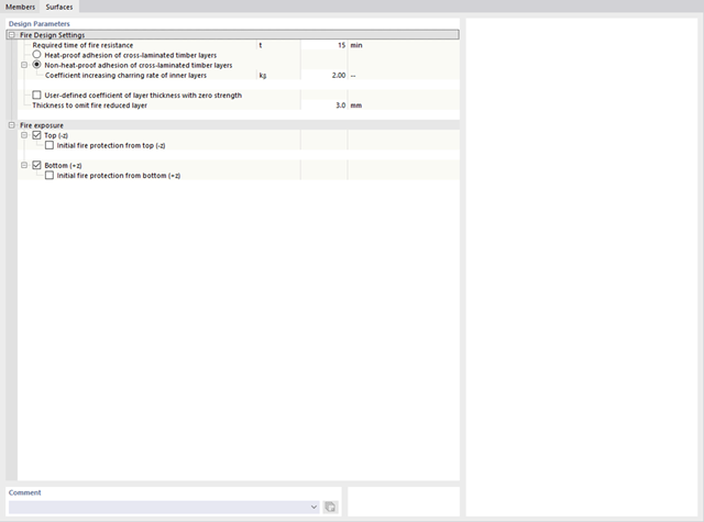
- Dowolna definicja czasu zwęglania
- W przypadku konstrukcji powierzchniowych (drewno klejone krzyżowo) można obliczyć z przyczepnością lub bez
- Bezpłatna, zdefiniowana przez użytkownika specyfikacja parametrów pożaru
- Uwzględnienie różnych długości efektywnych do obliczania odporności ogniowej
- Opcjonalne obliczenia dla 'ściskania w poprzek włókien'
- Zintegrowane z RFEM/RSTAB graficzne wyświetlanie wyników, np. B. Stopień wykorzystania
- Pełna integracja wyników z protokołem wydruku programu RFEM/RSTAB
- 002373
- Ogólne informacje
- Projektowanie konstrukcji drewnianych RFEM 6
- Projektowanie konstrukcji drewnianych RSTAB 9
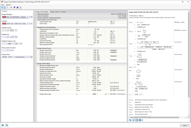
Program RFEM/RSTAB oferuje również szereg funkcji na wypadek pożaru. Program umożliwia automatyczne generowanie kombinacji obciążeń i wyników dla wyjątkowej sytuacji obliczeniowej w obliczeniach odporności ogniowej. Pręty, które mają zostać zwymiarowane wraz z odpowiednimi siłami wewnętrznymi, są importowane bezpośrednio z programu RFEM/RSTAB. Przechowywane są również wszystkie informacje o materiale i przekroju. Nie musisz'robić nic więcej.
Parametry istotne dla obliczeń odporności ogniowej można definiować poprzez przypisanie konfiguracji odporności ogniowej do obliczanych prętów i powierzchni. Ponadto można wprowadzić dalsze szczegółowe ustawienia, takie jak zdefiniowanie ekspozycji na ogień z jednej strony aż po wszystkie strony.
- 002374
- Ogólne informacje
- Projektowanie konstrukcji drewnianych RFEM 6
- Projektowanie konstrukcji drewnianych RSTAB 9
Jak zapewne wiesz, weryfikacje są przeprowadzane dla wybranych prętów z uwzględnieniem zdefiniowanego czasu zwęglania. Wszystkie niezbędne współczynniki i współczynniki redukcyjne są zapisywane w programie i uwzględniane przy określaniu nośności konstrukcji. Pozwala to zaoszczędzić dużo pracy.
Długości efektywne dla obliczeń pręta zastępczego są pobierane bezpośrednio z danych dotyczących wytrzymałości. Nie trzeba ich ponownie wprowadzać.
Po zakończeniu obliczeń program wyświetla w przejrzysty sposób obliczenia odporności ogniowej ze wszystkimi szczegółami wyników. Pozwala to na przejrzyste śledzenie wyników. Wyniki zawierają również wszystkie wymagane parametry, dzięki czemu można określić temperaturę elementu w czasie projektowania.
Oprócz wszystkich tych funkcji, program umożliwia zintegrowanie wszystkich tabel wyników i grafik, w tym wyników stanu granicznego nośności i użytkowalności, z globalnym protokołem wydruku programu RFEM/RSTAB, jako część wyników obliczeń stali.
- 002375
- Ogólne informacje
- Projektowanie konstrukcji drewnianych RFEM 6
- Projektowanie konstrukcji drewnianych RSTAB 9
W przypadku obliczeń zgodnie z Eurokodem 5 parametry załączników krajowych (NA) są zintegrowane dla następujących krajów:
-
 DIN EN 1995-1-1/NA:2014-07 (Niemcy)
 -
 ÖNORM EN 1995-1-1/NA:2019-06 (Austria)
 -
 SN EN 1995-1-1/NA:2015-03 (Szwajcaria)
 -
 BDS EN 1995-1-1/NA:20157-06 (Bułgaria)
 -
 BS EN 1995-1-1/NA:2019-09 (Wielka Brytania)
 -
 CEN EN 1995-1-1/2014-05 (Unia Europejska)
 -
 CYS EN 1995-1-1/NA:2019-06 (Cypr)
 -
 CZE EN 1995-1-1/NA:2015-05 (Republika Czeska)
 -
 DS EN 1995-1-1/NA:2019-09 (Dania)
 -
 ELOT EN 1995-1-1/NA:2010-01 (Grecja)
 -
 EVS EN 1995-1-1/NA:2015-11 (Estonia)
 -
 HRN EN 1995-1-1/NA:2015-03 (Chorwacja)
 -
 I S. EN 1995-1-1/NA:2014-05 (Irlandia)
 -
 ILNAS EN 1995-1-1/NA:2020-3 (Luksemburg)
 -
 IST EN 1995-1-1/NA:2014-09 (Islandia)
 -
 LST EN 1995-1-1/NA:2014-06 (Litwa)
 -
 LVS EN 1995-1-1/NA:2014-12 (Łotwa)
 -
 MSZ EN 1995-1-1/NA:2015-06 (Węgry)
 -
 NBN EN 1995-1-1/NA:2014-06 (Belgia)
 -
 NEN EN 1995-1-1/NA:2014-06 (Holandia)
 -
 NF EN 1995-1-1/NA:2020-04 (Francja)
 -
 NP EN 1995-1-1/NA:2014-09 (Portugalia)
 -
 NS EN 1995-1-1/NA:2014-08 (Norwegia)
 -
 PN EN 1995-1-1/NA:2014-07 (Polska)
 -
 SFS EN 1995-1-1/NA:2016-12 (Finlandia)
 -
 SIST EN 1995-1-1/NA:2018-01 (Słowenia)
 -
 SR EN 1995-1-1/NA:2014-12 (Rumunia)
 -
 SS EN 1995-1-1/NA:2018-02 (Singapur)
 -
 SS EN 1995-1-1/NA:2014-05 (Szwecja)
 -
 STN EN 1995-1-1/NA:2019-12 (Słowacja)
 -
 TKP EN 1995-1-1/NA:2019-09 (Białoruś)
 -
 UNE EN 1995-1-1/NA:2016-04 (Hiszpania)
 -
 UNI EN 1995-1-1/NA:2016-11 (Włochy)
- 002377
- Ogólne informacje
- Projektowanie konstrukcji drewnianych RFEM 6
- Projektowanie konstrukcji drewnianych RSTAB 9
Masz wiele możliwości w projektowaniu konstrukcji drewnianych. Dla prętów o zmiennym przekroju i zakrzywionych, możliwe jest uwzględnienie kątów nacięcia względem włókien, naprężeń rozciągających poprzecznych oraz zależnych od objętości promieni krzywizny. Aby obliczyć pole przekroju włókien, wytrzymałość na rozciąganie lub zginanie jest odpowiednio dostosowywana. Aby umożliwić również przeprowadzenie analizy stateczności metodą prętów zastępczych, wysokość do wyznaczenia długości efektywnej i długości wyboczeniowej została ustawiona jako odległość 0,65 × h od rzeczywistego punktu obliczeniowego.
- 002378
- Ogólne informacje
- Projektowanie konstrukcji drewnianych RFEM 6
- Projektowanie konstrukcji drewnianych RSTAB 9
Tutaj masz wolny wybór. Obliczenie ciśnienia w podporach można przeprowadzić w dowolnym punkcie dla obciążenia w kierunkach y i z przekroju. Użytkownik może dowolnie rozróżnić podpory wewnętrzne i zewnętrzne. Użytkownik może zdefiniować współczynnik kc,90 dla parcia prostopadłego do włókien (np. 1,75 dla drewna klejonego warstwowo). Jeżeli jest to dozwolone, długość podpory jest automatycznie zwiększana zgodnie ze specyfikacjami normy. Dzięki temu można przeprowadzić bardziej efektywne obliczenia przy minimalnym wysiłku.