Smoothing of Surface Internal Forces in RFEM

Technical Article

Back to Knowledge Base

KB 001606 | Glättung der Flächenschnittgrößen in RFEM

01
Example

02
Unsmoothed Results According to Mindlin (Left) and Kirchhoff (Right)

03
Smoothed Distribution of Internal Forces v-x and m-x According to Mindlin

04
Smoothed Distribution of Internal Forces v-x and m-x According to Kirchhoff

Back to Knowledge Base

4 November 2019

001606

Finite Element Analysis

When calculating a surface model, the internal forces are determined separately for each finite element. Since the element-by-element results usually represent a discontinuous distribution, RFEM performs smoothing of the internal forces that takes into account the influence of adjacent elements. The discontinuous distribution of internal forces is adjusted with this method. The result evaluation is thus clearer and easier.

You can select different options in the program to display unsmoothed or smoothed results. They are described in the RFEM manual. Smoothing options to evaluate surface internal forces and stresses are also explained in this technical article. The following article uses an example to illustrate how the internal forces in finite elements for smoothing are used to determine the values. In addition to the position of a finite element, the plate theory - Mindlin or Kirchhoff - plays a role in this process.

Example: Plate According to Mindlin and Kirchhoff

Image 01 - Example

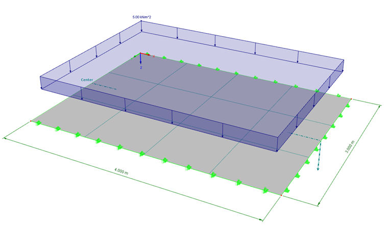
A plate with the dimensions 4 m ⋅ 3 m is created as a two-dimensional model. The plate is hinged on both sides to the shorter boundary lines. The rotation of the longer boundary lines is restrained by a restraint. To avoid transversal strain effects, Poisson's ratio of the material is set to zero. To compare the determination of internal forces according to the plate-bending theories of Kirchhoff and Mindlin, a plate thickness of 80 cm is selected. Thus, the ratio d/L = 0.2 is given in the limit zone between the two bending theories (see https://www.dlubal.com/en/support-and-learning/support/faq/003158).

To keep it simple, the mesh size of the FE mesh is set to 1 m. Thus, there are 4 ⋅ 3 finite elements.

A load of p = 5 kN/m² acts on the plate. The self-weight is not applied in the load case.

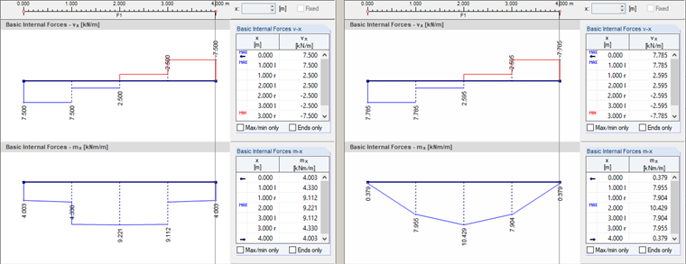
Unsmoothed Internal Forces

The results of the computation kernel for the internal forces v_x and m_x are considered for a longitudinal section running in the center of the plate. The distribution of the unsmoothed internal forces element by element can be represented by the "Not Continuous" display option. According to the bending theories of Mindlin and Kirchhoff, the diagrams shown in Figure 02 are available.

Image 02 - Unsmoothed Results According to Mindlin (Left) and Kirchhoff (Right)

Standard Smoothing for Internal Nodes

For FE nodes that lie within a surface, the arithmetic mean is first formed from the nodal values of the adjacent finite elements. For this approach, the elements must lie in a surface and on the same side of a possible internal line. The node must not be a user-defined node in the surface.

For the location of discontinuity at x = 1.00 m, these values are the following internally (the result of this step is not available for the output).

Mindlin:

Formula 1

$v_{x} (1) = \frac{7.5 2.5}{2} = 5 m_{x} (1) = \frac{8.772 5.351}{2} = 7.061$

Kirchhoff:

Formula 2

$v_{x} (1) = \frac{7.785 2.595}{2} = 5.19 m_{x} (1) = \frac{7.954 7.904}{2} = 7.929$

Smoothing for Edge Nodes

At the edges of a surface ("Continuous within surfaces" smoothing option) or a model ("Continuous Total"), there are no adjacent finite elements that could be used for averaging the nodal values. Therefore, a different approach is used, which is performed in two steps.

In the first step, the averaged values are calculated for those nodes that are not located on the edge of a surface or the model. The values of the nodes at the edges are calculated in such a way that the original values remain in the centers of the finite elements. In the second step, the averaged values for the edge nodes are determined.

The following values result for the edge node at x = 0.00 m.

Mindlin:

Formula 3

$v_{x} (0) = 7.5 (7.5 - 5) = 10 m_{x} (0.5) = \frac{5.351 2.982}{2} = 4.167 m_{x} (0) = 4.167 (4.167 - 7.061) = 1.272$

Kirchhoff:

Formula 4

$v_{x} (0) = 7.785 (7.785 - 5.19) = 10.381 m_{x} (0.5) = \frac{7.954 0.379}{2} = 4.167 m_{x} (0) = 4.167 (4.167 - 7.929) = 0.404$

Shear Forces

According to Mindlin, the shear forces are calculated as the first derivative of the deflection.

Formula 5

$v_{x} = \frac{5 \cdot G \cdot h}{6} \cdot (\frac{\partial w}{\partial x} Φ_{y}) v_{y} = \frac{5 \cdot G \cdot h}{6} \cdot (\frac{\partial w}{\partial y} Φ_{x})$

These values are determined by the calculation kernel and used directly. The smoothing of shear forces is then carried out as described above, depending on the position of the FE node in the surface.

In the bending theory according to Kirchhoff, the shear forces are calculated as the third derivative of the deflection.

Formula 6

$v_{x} = - \frac{E \cdot h^{3}}{12 \cdot (1 - μ^{2})} \cdot (\frac{\partial^{3} w}{\partial x^{3}} \frac{\partial^{3} w}{\partial x \partial y^{2}}) v_{y} = - \frac{E \cdot h^{3}}{12 \cdot (1 - μ^{2})} \cdot (\frac{\partial^{3} w}{\partial y^{3}} \frac{\partial^{3} w}{\partial x^{2} \partial y})$

This value determination using the third derivative results in a considerable loss of accuracy. For this reason, the shear forces of the computation kernel are not used, but determined from the derivations of the moments by an improved approach.

Formula 7

$v_{x} = \frac{\partial m_{x}}{\partial x} \frac{\partial m_{xy}}{\partial y} v_{y} = \frac{\partial m_{y}}{\partial y} \frac{\partial m_{xy}}{\partial x}$

The moments m_x, m_y, and m_xy in the equations represent the smoothed values that are determined according to the methods described above. This results in more accurate values for the shear forces than calculating them with the computation kernel.

Formula 8

$v_{x} {(0)}^{} = v_{x} {(1)}^{-} = 7.929 - 0.404 = 7.525 v_{x} {(1)}^{} = v_{x} {(2)}^{-} = 10.429 - 7.929 = 2.5 v_{x} (1) = \frac{7.525 2.5}{2} = 5.013 v_{x} (0) = 7.525 7.525 - 5.013 = 10.038$

Moments

While the moment values in the integration points correspond to the theoretical values, the extrapolation leads to a loss of accuracy when using the hyperbolic paraboloid function for smoothing. A hyperbolic paraboloid only approximates the moment distribution in the element. For this reason, an improved algorithm is used that replaces the extrapolation with an advanced shear force integral method. Since the distribution of shear force in the surface element is assumed to be the shape of a hyperbolic paraboloid (surface of the second order), the integral of this surface represents a surface of the third order, which displays the moment distribution with greater accuracy.

This approach corresponds to the equations described above for determining the shear forces via the derivatives of the moments. The moments are then determined with the following equations.

Formula 9

$m_{x} = \int (v_{x} - \frac{\partial m_{xy}}{\partial y}) dx m_{x, 0} m_{y} = \int (v_{y} - \frac{\partial m_{xy}}{\partial x}) dy m_{y, 0}$

The integration constants m_x,0 and m_y,0 are calculated from the conditions of the value in the center of the member.

Formula 10

$m_{x, C} = \frac{\int_{S} m_{x} dS}{S} m_{y, C} = \frac{\int_{S} m_{y} dS}{S}$

S represents the surface of the element.

The values of the internal forces are determined by the methods described above; the integrals, by a numerical integration. The moments thus determined are then smoothed according to the method for internal nodes or edge nodes.

In the bending theory according to Mindlin, the following values result in this example.

First element:

Formula 11

$v_{x} (x) = 10 - 5 x m_{x} (x) = \int v_{x} dx m_{x, 0} = 10 x - \frac{5}{2} x^{2} m_{x, 0} m_{x, C} = m_{x} (0.5) = 4.167 = \int_{0}^{1} 10 x - \frac{5}{2} x^{2} m_{x, 0} = {[\frac{10}{2} x^{2} - \frac{5}{6} x^{3} m_{x, 0} x]}_{0}^{1} = 4.167 m_{x, 0} m_{x, 0} = m_{x} (0) = 4.167 - 4.167 = 0 m_{x} {(1)}^{-} = 10 - \frac{5}{2} 0 = 7.5$

Second element:

Formula 12

$v_{x} (x) = 5 - 5 x m_{x} (x) = \int v_{x} dx + m_{x, 0} = 5 x - \frac{5}{2} x^{2} + m_{x, 0} m_{x, C} = m_{x} (1.5) = 9.167 = \int_{0}^{1} 5 x - \frac{5}{2} x^{2} + m_{x, 0} = {[\frac{5}{2} x^{2} - \frac{5}{6} x^{3} + m_{x, 0} x]}_{0}^{1} = 1.667 + m_{x, 0} m_{x, 0} = m_{x} (1)^{+} = 9.167 - 1.667 = 7.5 m_{x} (1) = \frac{m_{x} (1)^{-} + m_{x} (1)^{+}}{2} = \frac{7.5 + 7.5}{2} = 7.5$

Image 03 - Smoothed Distribution of Internal Forces v-x and m-x According to Mindlin

The following values are obtained for the bending theory according to Kirchhoff.

First element:

Formula 13

$v_{x} (x) = 10.038 - 5.025 x m_{x} (x) = \int v_{x} dx m_{x, 0} = 10.038 x - \frac{5.025}{2} x^{2} m_{x, 0} m_{x, C} = m_{x} (0.5) = 4.167 = \int_{0}^{1} 10.038 x - \frac{5.025}{2} x^{2} m_{x, 0} = {[\frac{10.038}{2} x^{2} - \frac{5.025}{6} x^{3} m_{x, 0} x]}_{0}^{1} = 4.182 m_{x, 0} m_{x, 0} = m_{x} (0) = 4.167 - 4.182 = - 0.015 m_{x} {(1)}^{-} = 10.038 - \frac{5.025}{2} - 0.015 = 7.511$

Second element:

Formula 14

$v_{x} (x) = 5.013 - 5.013 x m_{x} (x) = \int v_{x} dx + m_{x, 0} = 5.013 x - \frac{5.013}{2} x^{2} + m_{x, 0} m_{x, C} = m_{x} (1.5) = 9.167 = \int_{0}^{1} 5.013 x - \frac{5.013}{2} x^{2} + m_{x, 0} = {[\frac{5.013}{2} x^{2} - \frac{5.013}{6} x^{3} + m_{x, 0} x]}_{0}^{1} = 1.671 + m_{x, 0} m_{x, 0} = m_{x} (1)^{+} = 9.167 - 1.671 = 7.496 m_{x} (1) = \frac{m_{x} (1)^{-} + m_{x} (1)^{+}}{2} = \frac{7.511 + 7.496}{2} = 7.503$

Image 04 - Smoothed Distribution of Internal Forces v-x and m-x According to Kirchhoff

In the smoothing process, the steps described above are performed gradually in the program. The smoothed values can be displayed graphically with the display option "Continuous within Surfaces".

Author

Dipl.-Ing. (FH) Robert Vogl

Technical Editor, Product Engineering & Customer Support

Mr. Vogl creates and maintains the technical documentation. In addition, he is involved in the development of the SHAPE-THIN program and provides customer support.