


Introduction
In computational modeling and simulation, especially in the field of fluid dynamics and wind load analysis, it is essential to quantitatively assess the accuracy of numerical results against reference data. While hit rate methods offer a binary evaluation based on predefined tolerance thresholds, they may overlook the overall distribution and magnitude of deviations. To address this, the normalized mean squared error e2 provides a complementary approach by delivering a continuous, scale-independent measure of model performance as mentioned in Section 5.3.2 of the WTG-Merkblatt M3. This article explores the definition, advantages, and limitations of using e2 as a validation criterion.
Definition of the Normalized Mean Squared Error
In the context of validating simulated data against reference measurements, one alternative to hit rate analysis is the calculation of the normalized mean squared error, denoted as e2. This approach offers a more continuous and quantitative measure of deviation between predicted values Pi and observed values Oi. The formula is defined as:
This ratio-based expression evaluates the squared deviations normalized by the magnitude of the observed values. It provides a dimensionless error metric that allows for better comparability across datasets with different scales.
Advantages of e2 in Model Evaluation
- Model Calibration: The normalized mean squared error can be directly related to the model factor, making it useful for calibration tasks.
- Applicability to Small Datasets: Unlike hit rate methods that require statistically large datasets, e2 can be meaningfully applied even with smaller samples.
- Quantitative Precision: A value of e2≤0.01 is considered a good benchmark for accurate simulation performance, indicating that only 1% of the total energy in the observed signal is not captured by the model.
Limitations
One drawback of the e2 method is its sensitivity to outliers. Significant individual deviations can increase the error disproportionately, even if the majority of the values are well predicted. Therefore, in critical applications, it is advisable to complement this metric with threshold-based hit rate criteria to ensure a more robust validation.
Example: Evaluation of the Normalized Mean Squared Error (𝑒2) for 12 Measurement Points on a Surface
Let's consider 12 measured points with reference values Oi and corresponding simulation values Pi:
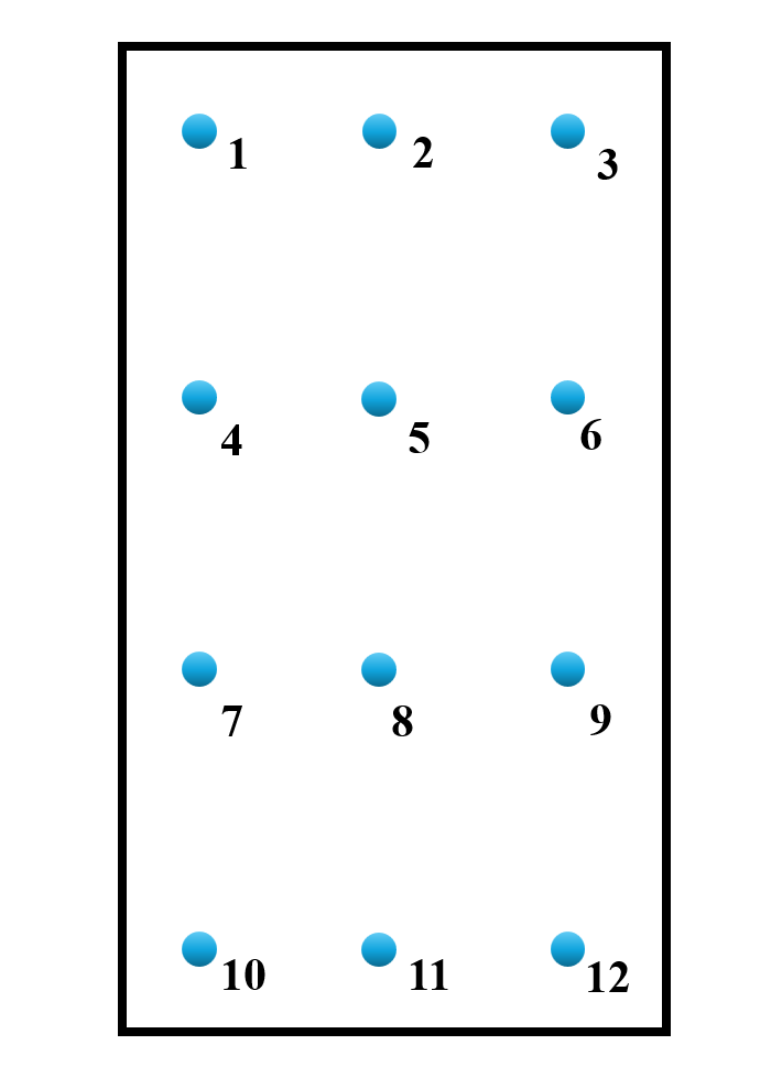
Table 1: 12 Measurement Points Info
| Point (i) | Reference Value (Oi) | Simulated Value (Pi) |
|---|---|---|
| 1 | 0.72 | 0.75 |
| 2 | 0.68 | 0.70 |
| 3 | 0.81 | 0.85 |
| 4 | 0.77 | 0.73 |
| 5 | 0.66 | 0.69 |
| 6 | 0.74 | 0.71 |
| 7 | 0.85 | 0.80 |
| 8 | 0.70 | 0.66 |
| 9 | 0.81 | 0.88 |
| 10 | 0.76 | 0.69 |
| 11 | 0.82 | 0.75 |
| 12 | 0.69 | 0.80 |
So we can calculate e2 with the following formula:
Normalized Mean Squared Error: 𝑒2=0.0055
It meets the minimum requirement (e2≤0.01) for validating mean values.
Conclusion
The 𝑒2 metric is a powerful tool for assessing the overall fidelity of simulation models, particularly in pressure or force coefficient evaluations in CFD validation studies. When used appropriately, it provides a reliable quantitative basis for verifying model performance and can complement categorical criteria like hit rate analysis for a more comprehensive quality assessment.