
As you've already learned, the results of a Modal Analysis load case are displayed in the program after a successful calculation. You can thus immediately see the first mode shape graphically or as an animation. You can also easily adjust the representation of the mode shape standardization. Do that directly in the Results navigator, where you have one of four options for the visualization of the mode shapes available for the selection:
- Scaling the value of the mode shape vector uj to 1 (considers the translation components only)
- Selecting the maximum translational component of the eigenvector and setting it to 1
- Considering the entire eigenvector (including the rotation components), selecting the maximum, and setting it to 1
- Setting the modal mass mi for each mode shape to 1 kg
You can find a detailed explanation of the mode shape standardization in the OnlineManual here.

Is the calculation finished? The results of the modal analysis are then available both graphically and in tables. Display the result tables for the load case or the load cases of the modal analysis. Thus, you can see the eigenvalues, angular frequencies, natural frequencies, and natural periods of the structure at first glance. The effective modal masses, modal mass factors, and participation factors are also clearly displayed.

You can perform the calculation of the warping torsion on the entire system. Thus, you consider the additional 7th degree of freedom in the member calculation. The stiffnesses of the connected structural elements are automatically taken into account. It means, you don't need to define equivalent spring stiffnesses or support conditions for a detached system.
You can then use the internal forces from the calculation with warping torsion in the add-ons for the design. Consider the warping bimoment and the secondary torsional moment, depending on the material and the selected standard. A typical application is the stability analysis according to the second-order theory with imperfections in steel structures.
Did you know that The application is not limited to thin-walled steel cross-sections. Thus, it is possible for you, for example, to perform the calculation of the ideal overturning moment of beams with solid timber cross-sections.
Compared to the RF-/STEEL Warping Torsion add-on module (RFEM 5 / RSTAB 8), the following new features have been added to the Torsional Warping (7 DOF) add-on for RFEM 6 / RSTAB 9:
- Complete integration into the environment of RFEM 6 and RSTAB 9
- 7th degree of freedom is directly taken into account in the calculation of members in RFEM/RSTAB on the entire system
- No more need to define support conditions or spring stiffnesses for calculation on the simplified equivalent system
- Combination with other add-ons is possible, for example for the calculation of critical loads for torsional buckling and lateral-torsional buckling with stability analysis
- No restriction to thin-walled steel sections (it is also possible to calculate ideal overturning moments for beams with massive timber sections, for example)

Are you ready for the evaluation? Use the calculation diagrams, which show the distribution of a specific result during the calculation.
You can freely define the layout of the vertical and horizontal axes of the calculation diagram. This allows you, for example, to consider the settlement distribution of a certain node, depending on the load.

Is your goal to determine the number of mode shapes? The program offers you two methods for this. On the one hand, you can manually define the number of the smallest mode shapes to be calculated. In this case, the number of available mode shapes depends on the degrees of freedom (that is, the number of free mass points multiplied by the number of directions in which the masses act). However, it is limited to 9999. On the other hand, you can set the maximum natural frequency the way that the program determined the mode shapes automatically until reaching the natural frequency set.
- Consideration of 7 local deformation directions (ux, uy, uz, φx, φy, φz, ω) or 8 internal forces (N, Vu, Vv, Mt,pri, Mt,sec, Mu, Mv, Mω) when calculating member elements
- Usable in combination with a structural analysis according to linear static, second-order, and large deformation analysis (imperfections can also be taken into account)
- In combination with the Stability Analysis add-on, allows you to determine critical load factors and mode shapes of stability problems such as torsional buckling and lateral-torsional buckling
- Consideration of end plates and transverse stiffeners as warping springs when calculating I-sections with automatic determination and graphical display of the warping spring stiffness
- Graphical display of the cross-section warping of members in the deformation
- Full integration with RFEM and RSTAB
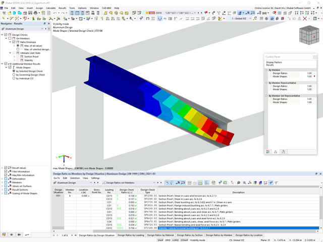
Did you use the eigenvalue solver of the add-on to determine the critical load factor within the stability analysis? In this case, you can then display the governing mode shape of the object to be designed as a result.
The Aluminum Design add-on provides you with further options. Here you can also design general cross-sections that are not predefined in the cross-section library. For example, create a cross-section in the RSECTION program and then import it into RFEM/RSTAB. Depending on the design standard used, you can select from various design formats. This includes, for example, the equivalent stress analysis.
With a license for RSECTION and Effective Sections, you can also perform the design checks while taking into account the effective cross-section properties according to EN 1993‑1‑5.

Do you want to model and analyze the behavior of a soil solid? To ensure this, special suitable material models have been implemented in RFEM.
You can use the modified Mohr-Coulomb model with a linear-elastic ideal-plastic model or a nonlinear elastic model with an oedometric stress-strain relation. The limit criterion, which describes the transition from the elastic area to that of the plastic flow, is defined according to Mohr-Coulomb.

Compared to the RF‑SOILIN add-on module (RFEM‑5), the following new features have been added to the Geotechnical Analysis add-on for RFEM 6:
- Creation of the layered soil as a 3D model from the entirety of the defined soil samples
- Recognized material law according to Mohr-Coulomb for soil simulation
- Graphical and tabular output of stresses and strains at any depth of the soil
- Optimal consideration of the soil-structure interaction on the basis of an overall model

The Concrete Design add-on allows you to perform the seismic design of reinforced concrete members according to EC 8. This includes, among other things, the following functionalities:
- Seismic design configurations
- Differentiation of the ductility classes DCL, DCM, DCH
- Option to transfer the behavior factor from a dynamic analysis
- Check of the limit value for the behavior factor
- Capacity design checks of "Strong column - weak beam"
- Detailing and particular rules for curvature ductility factor
- Detailing and particular rules for local ductility

You can select several methods that are available for the eigenvalue analysis:
- Direct Methods
- The direct methods (Lanczos [RFEM], roots of characteristic polynomial [RFEM], subspace iteration method [RFEM/RSTAB], and shifted inverse iteration [RSTAB]) are suitable for small to medium-sized models. You should only use these fast solver methods if your computer has a larger amount of memory (RAM).
- ICG Iteration Method (Incomplete Conjugate Gradient [RFEM])
- In contrast, this method only requires a small amount of memory. Eigenvalues are determined one after the other. It can be used to calculate large structural systems with few eigenvalues.
Use the Structure Stability add-on to perform a nonlinear stability analysis using the incremental method. This analysis delivers close-to-reality results also for nonlinear structures. The critical load factor is determined by gradually increasing the loads of the underlying load case until the instability is reached. The load increment takes into account nonlinearities such as failing members, supports and foundations, and material nonlinearities. After increasing the load, you can optionally perform a linear stability analysis on the last stable state in order to determine the stability mode.

The soil solids that you want to analyze are summarized in soil massifs.
Use the soil samples as a basis for a definition of the respective soil massif. This way, the program allows for user-friendly generation of the massif, including the automatic determination of the layer interfaces from the sample data, as well as the groundwater level and the boundary surface supports.
Soil massifs provide you with the option to specify a target FE mesh size independently of the global setting for the rest of the structure. You can thus consider the various requirements of the building and soil in the entire model.

Your data are always documented in a multilingual printout report. You can adjust the content at any time and save it as a template. You can also add graphics, texts, MathML formulas, and PDF documents to your report with just a few clicks.

- Stability analyses for flexural buckling, torsional buckling, and flexural-torsional buckling under compression
- Lateral-torsional buckling analysis of the structural components subjected to moment loading
- Import of the effective lengths from the calculation using the Structure Stability add-on
- Graphical input and check of the defined nodal supports and effective lengths for stability analysis
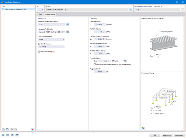
- Depending on the standard, a choice between user-defined input of Mcr, analytical method from the standard, and use of internal eigenvalue solver
- Consideration of a shear panel and a rotational restraint when using the eigenvalue solver
- Graphical display of a mode shape if the eigenvalue solver was used
- Stability analysis of structural components with the combined compression and bending stress, depending on the design standard
- Comprehensible calculation of all necessary coefficients, such as interaction factors
- Alternative consideration of all effects for the stability analysis when determining internal forces in RFEM/RSTAB (second-order analysis, imperfections, stiffness reduction, possibly in combination with the Torsional Warping (7 DOF) add-on)
Compared to the RF‑/ALUMINUM add-on module (RFEM 5 / RSTAB 8), the following new features have been added to the Aluminum Design add-on for RFEM 6 / RSTAB 9:
- In addition to Eurocode 9, the US standard ADM 2020 is integrated.
- Consideration of the stabilizing effect of purlins and sheets by rotational restraints and shear panels
- Graphical display of the results in the gross section
- Output of the used design check formulas (including a reference to the used equation from the standard)

- You can activate or deactivate the use of torsional warping in the Add-ons tab of the model's Base Data.
- After activating the add-on, the user interface in RFEM is extended by some new entries in the navigator, tables, and dialog boxes.

Compared to the RF‑/STABILITY (RFEM 5) and RSBUCK (RSTAB 8) add-on modules, the following new features have been added to the Structure Stability add-on for RFEM 6 / RSTAB 9:
- Activation as a property of a load case or a load combination
- Automated activation of the stability calculation via combination wizards for several load situations in one step
- Incremental load increase with user-defined termination criteria
- Modification of the mode shape normalization without recalculation
- Result tables with filter option
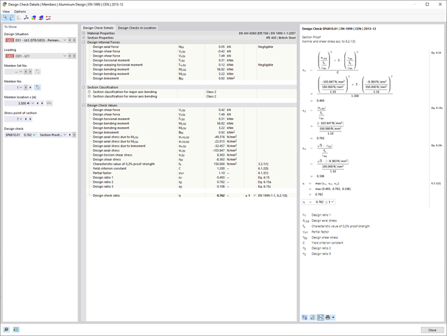
The Torsional Warping (7 DOF) add-on allows you to perform the calculation of member structures in RFEM and RSTAB, taking into account the cross-section warping. You can consider all internal forces (N, Vu, Vv, Mt,pri, Mt,sec, Mu, Mv, Mω) determined in this way in the equivalent stress analysis of the aluminum design. Please Note: This feature is not yet available for the design standard ADM 2020.

Have you already discovered the tabular and graphical output of masses in mesh points? That's right, this is also part of the modal analysis results in RFEM 6. This way, you can check the imported masses that depend on various settings of the modal analysis. They can be displayed in the Masses in Mesh Points tab of the Results table. The table provides you with an overview of the following results: Mass - Translational Direction (mX, mY, mZ), Mass - Rotational Direction (mφX, mφY, mφZ), and the Sum of Masses. Would it be best for you to have a graphical evaluation as quickly as possible? Then you can also graphically display the masses in mesh points.

Did you know that Equivalent static loads are generated separately for each relevant eigenvalue and excitation direction. These loads are saved in a load case of the Response Spectrum Analysis type and RFEM/RSTAB performs a linear static analysis.
.png?mw=640&hash=55038d2a1591f62179796666cb9b2fede0274e19)
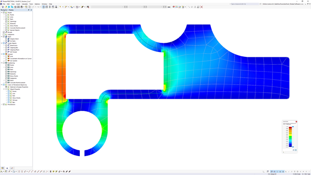
A graphical and tabular output of the results for deformations, stresses, and strains helps you when determining the soil solids. To achieve this, use the special filter criteria for targeted selection of results.
The program doesn't leave you alone with the results. If you want to graphically evaluate the results in the soil solids, you can use the guide objects. For example, you can define clipping planes. This allows you to view the corresponding results in any plane of the soil solid.
And not just that. The utilization of result sections and clipping boxes facilitates the precise graphical analysis of the soil solid.
You already know that it is possible to model and analyze a soil and a structure in the entire model. As a result, you have explicitly taken into account the soil-structure interaction. By modifying a component, you achieve the immediate correct consideration in the analysis as well as in the results for the entire system of the soil and structure.

As the first results, the program presents you with the critical load factors. You can then perform an evaluation of stability risks. For member models, the resulting effective lengths and critical loads of the members are displayed to you in tables.
Use the next result window to check the normalized eigenvalues sorted by node, member, and surface. The eigenvalue graphic allows you to evaluate the buckling behavior. This makes it easier for you to take countermeasures.

Did you know? You can enter the soil layers that you have obtained from the subsoil expertises done in the locations into the program in the form of soil samples. Assign the explored soil materials, including their material properties, to the layers.
For the definition of the samples, you can enter the data in tables as well as in the respective editing dialog box. Furthermore, you can also specify the groundwater level in the soil samples.
Entering soil layers for soil samples is performed in a clearly arranged dialog box. A corresponding graphical representation supports clarity and makes checking the input user-friendly.
An extensible database facilitates the selection of soil material properties. The Mohr-Coulomb model as well as a nonlinear model with stress and strain dependent stiffness are available for a realistic modeling of the soil material behavior.
You can define any number of soil samples and layers. The soil is generated from all entered samples using 3D solids. Assignment to the structure is carried out using coordinates.
The soil body is calculated according to the nonlinear iterative method. The calculated stresses and settlements are displayed graphically and in tables.

The load cases of the type Response Spectrum Analysis contain the generated equivalent loads. First, the modal contributions have to be superimposed with the SRSS or CQC rule. In this case, you can use the signed results based on the dominant mode shape.
Afterwards, the directional components of earthquake actions are combined with the SRSS or the 100% / 30% rule.
Compared to the RF-/DYNAM Pro - Equivalent Loads add-on module (RFEM 5 / RSTAB 8), the following new features have been added to the Response Spectrum Analysis add-on for RFEM 6 / RSTAB 9:
- Response spectra of numerous standards (EN 1998, DIN 4149, IBC 2018, and so on)
- User-defined response spectra or those generated from accelerograms
- Direction-relative response spectrum approach
- Results are stored centrally in a load case with underlying levels to ensure clarity
- Accidental torsional actions can be taken into account automatically
- Automatic combinations of seismic loads with the other load cases for use in an accidental design situation
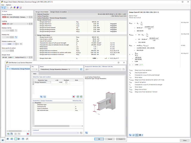
You know for sure that when connecting tension-loaded components with bolted connections, you need to consider the cross-section reduction due to the bolt holes in the ultimate limit state design. The structural analysis programs also have a solution for this. In the Aluminum Design add-on, you can enter a member local section reduction for this. Enter the reduction of the cross-section as an absolute value or as a percentage of the total area at all relevant locations.