
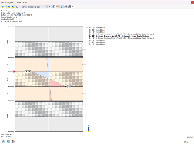
You have the option to perform the fire resistance design of surfaces using the reduced cross-section method. The reduction is applied over the surface thickness. It is possible to perform the design checks for all timber materials allowed for the design.
For cross-laminated timber, depending on the type of adhesive, you can select whether it is possible for individual carbonized layer parts to fall off, and whether you can expect increased charring in certain layer areas.
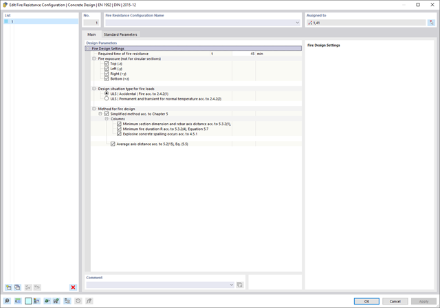
The Concrete Design add-on provides you with the option to perform the simplified fire resistance design according to EN 1992‑1‑2 for columns (Section 5.3.2) and beams (Section 5.6).
The following design checks are available for the simplified fire resistance design:
- Columns: Minimum cross-sectional dimensions for rectangular and circular sections according to Table 5.2a as well as Equation 5.7 for calculating time of fire exposure
- Beams: Minimum dimensions and center distances according to Table 5.5 and Table 5.6
You can determine the internal forces for the fire resistance design according to two methods.
- 1 Here, the internal forces of the accidental design situation are included directly into the design.
- 2 The internal forces of the design at normal temperature are reduced by the factor Eta,fi (ηfi), then used in the fire resistance design.
Furthermore, it is possible to modify the axis distance according to Eq. 5.5.
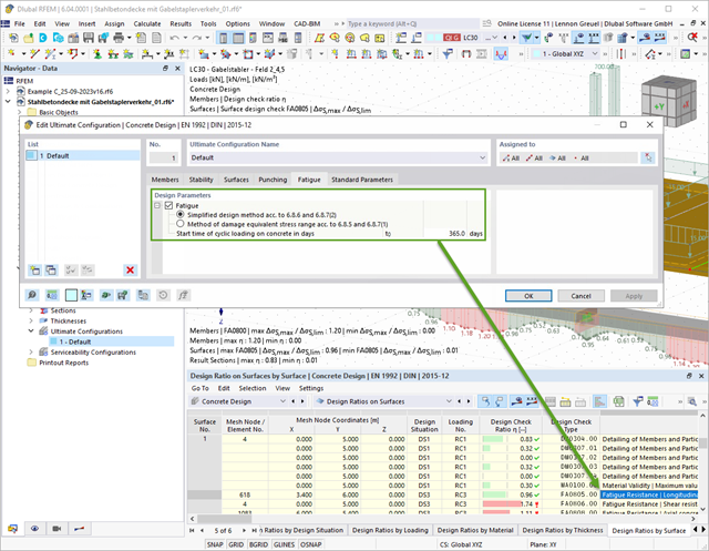
With the Concrete Design add-on, you can perform the fatigue design of members and surfaces according to EN 1992‑1‑1, Chapter 6.8.
For the fatigue design, you can optionally select two methods or design levels in the design configurations:
- Design Level 1: Simplified design according to 6.8.6 and 6.8.7(2): The simplified design is performed for frequent action combinations according to EN 1992‑1‑1, Chapter 6.8.6 (2), and EN 1990, Eq. (6.15b) with the traffic loads relevant in the serviceability state. A maximum stress range according to 6.8.6 is designed for the reinforcing steel. The concrete compressive stress is determined by means of the upper and lower allowable stress according to 6.8.7(2).
- Design Level 2: Design of damage equivalent stress acc. to 6.8.5 and 6.8.7(1) (simplified fatigue design): The design using damage equivalent stress ranges is performed for the fatigue combination according to EN 1992‑1‑1, Chapter 6.8.3, Eq. (6.69) with the specifically defined cyclic action Qfat.

The Concrete Design add-on allows you to perform the seismic design of reinforced concrete members according to EC 8. This includes, among other things, the following functionalities:
- Seismic design configurations
- Differentiation of the ductility classes DCL, DCM, DCH
- Option to transfer the behavior factor from a dynamic analysis
- Check of the limit value for the behavior factor
- Capacity design checks of "Strong column - weak beam"
- Detailing and particular rules for curvature ductility factor
- Detailing and particular rules for local ductility
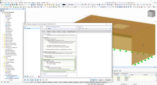
The Concrete Design add-on allows you to design fiber-reinforced concrete components according to the guideline "DAfStb Steel Fiber-Reinforced Concrete".
You can use this option for the design according to EN 1992‑1‑1. The design according to the DAfStb guideline is carried out once the concrete of the "Fiber Concrete" type has been assigned to the reinforced structural component.
Go to Explanatory Video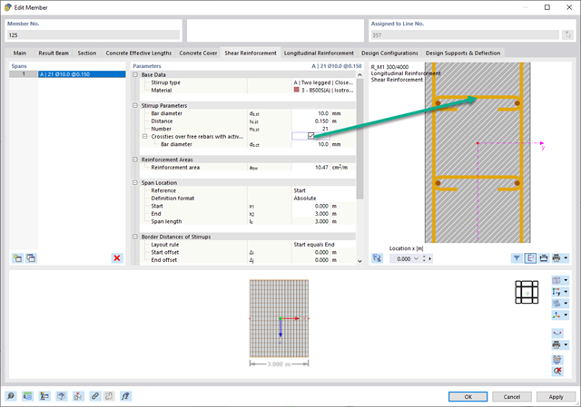
In the "Shear Reinforcement" tab, you can select the option "Cross-ties over free rebars with active selection in graphic". It allows you to arrange additional cross-ties on free rebars of the longitudinal reinforcement.
You can activate or deactivate the position of the cross-ties in the Info Graphic. The cross-ties are applied for the ultimate limit state design and the structural design checks. They are available for the design according to EN 1992‑1‑1.
Go to Explanatory Video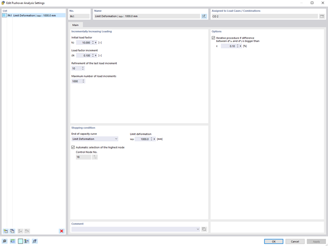
The pushover analysis is managed by a newly introduced analysis type in the load combinations. Here, you have access to the selection of the horizontal load distribution and direction, the selection of a constant load, the selection of the desired response spectrum for the determination of the target displacement, and the pushover analysis settings tailored to the pushover analysis.
In the pushover analysis settings, you can modify the increment of the increasing horizontal load and specify the stopping condition for the analysis. Furthermore, it is possible to easily adjust the precision for the iterative determination of the target displacement.
- Consideration of nonlinear component behavior using plastic standard hinges for steel (FEMA 356, EN 1998‑3) and nonlinear material behavior (masonry, steel - bilinear, user-defined working curves)
- Direct import of masses from load cases or combinations for the application of constant vertical loads
- User-defined specifications for the consideration of horizontal loads (standardized to a mode shape or uniformly distributed over the height of the masses)
- Determination of a pushover curve with selectable limit criterion of the calculation (a collapse or limit deformation)
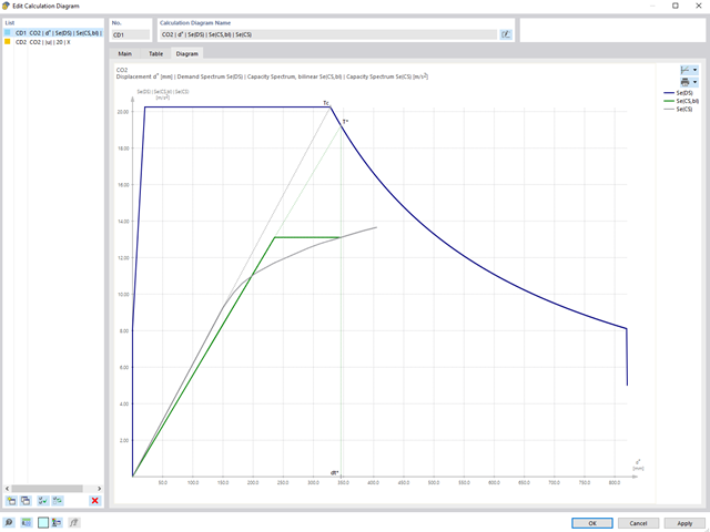
- Transformation of the pushover curve into the capacity spectrum (ADRS format, single degree of freedom system)
- Bilinearization of the capacity spectrum according to EN 1998‑1:2010 + A1:2013
- Transformation of the applied response spectrum into the required spectrum (ADRS format)
- Determination of target displacement according to EC 8 (the N2 method according to Fajfar 2000)
- Graphical comparison of the capacity and required spectrum
- Graphical evaluation of the acceptance criteria of predefined plastic hinges
- Result display of the values used in the iterative calculation of the target displacement
- Access to all results of the structural analysis in the individual load levels
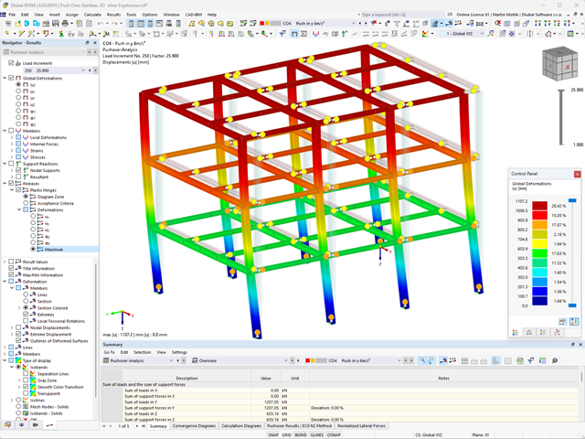
During the calculation, the selected horizontal load is increased in load steps. A static nonlinear analysis is carried out for each load step until reaching the specified limit condition.
The results of the pushover analysis are extensive. On one hand, the structure is analyzed for its deformation behavior. This can be represented by a force-deformation line of the system (a capacity curve). On the other hand, the response spectrum effect can be displayed in the ADRS display (Acceleration-Displacement Response Spectrum). The target displacement is automatically determined in the program based on these two results. The process can be evaluated graphically and in tables.
The individual acceptance criteria can then be graphically evaluated and assessed (for the next load step of the target displacement, but also for all other load steps). The results of the static analysis are also available for the individual load steps.
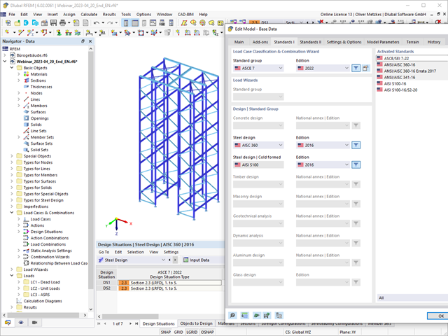
The design of cold-formed steel members according to the AISI S100-16 / CSA S136-16 is available in RFEM 6. Design can be accessed by selecting “AISC 360” or “CSA S16” as the standard in the Steel Design Add-on. “AISI S100” or “CSA S136” is then automatically selected for the cold-formed design.
RFEM applies the Direct Strength Method (DSM) to calculate the elastic buckling load of the member. The Direct Strength Method offers two types of solutions, numerical (Finite Strip Method) and analytical (Specification). The FSM signature curve and buckling shapes can be viewed under Sections.
Do you work with the structural components consisting of slabs? In that case, you have to perform the shear force design with the requirements of punching shear design, for example, according to 6.4, EN 1992‑1‑1. In addition to floor slabs, you can also design foundation slabs in this way.
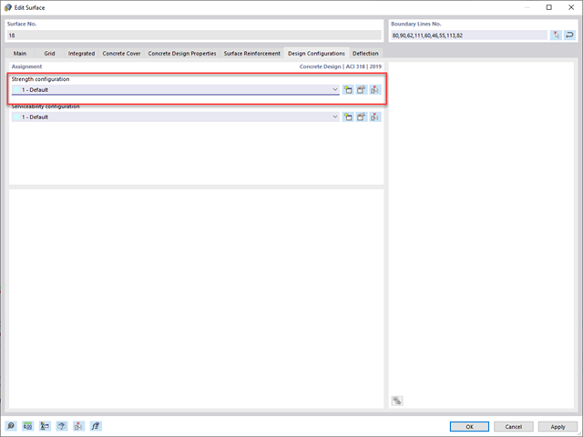
In the Ultimate Configuration for concrete design, you can define the punching design parameters for the selected nodes.
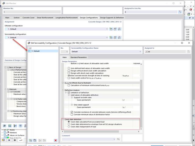
Various design parameters of the cross-sections can be adjusted in the serviceability limit state configuration. The applied cross-section condition for the deformation and crack width analysis can be controlled there.
For this, the following settings can be activated:
- Crack state calculated from associated load
- Crack state determined as an envelope from all SLS design situations
- Cracked state of cross-section - independent of load

Have you already discovered the tabular and graphical output of masses in mesh points? That's right, this is also part of the modal analysis results in RFEM 6. This way, you can check the imported masses that depend on various settings of the modal analysis. They can be displayed in the Masses in Mesh Points tab of the Results table. The table provides you with an overview of the following results: Mass - Translational Direction (mX, mY, mZ), Mass - Rotational Direction (mφX, mφY, mφZ), and the Sum of Masses. Would it be best for you to have a graphical evaluation as quickly as possible? Then you can also graphically display the masses in mesh points.

As you've already learned, the results of a Modal Analysis load case are displayed in the program after a successful calculation. You can thus immediately see the first mode shape graphically or as an animation. You can also easily adjust the representation of the mode shape standardization. Do that directly in the Results navigator, where you have one of four options for the visualization of the mode shapes available for the selection:
- Scaling the value of the mode shape vector uj to 1 (considers the translation components only)
- Selecting the maximum translational component of the eigenvector and setting it to 1
- Considering the entire eigenvector (including the rotation components), selecting the maximum, and setting it to 1
- Setting the modal mass mi for each mode shape to 1 kg
You can find a detailed explanation of the mode shape standardization in the OnlineManual here.

Do you want to consider other loads as masses in addition to the static loads? The program allows that for nodal, member, line and surface loads. For this, you need to select the Mass load type when defining the load of interest. Define a mass or mass components in the X, Y, and Z directions for such loads. For nodal masses, you have an additional option to also specify moments of inertia X, Y, and Z in order to model more complex mass points.

It is often necessary to neglect masses. This is particularly the case when you want to use the output of the modal analysis for the seismic analysis. For this, 90% of the effective modal mass in each direction is required for the calculation. So you can neglect the mass in all fixed nodal and line supports. The program automatically deactivates the associated masses for you.
You can also manually select the objects whose masses are to be neglected for the modal analysis. We have shown the latter in the image for a better view. A user-defined selection is made the and the objects with their associated mass components are selected to neglect the masses.

When defining the input data for the modal analysis load case, you can consider a load case whose stiffnesses represent the initial position for the modal analysis. How do you do that? As shown in the image, select the "Consider initial state from" option. Now, open the "Initial State Settings" dialog box and define the type Stiffness as the initial state. In this load case, as of which is the initial state taken into account, you can consider the stiffness of the structural system when the tension members fail. The purpose of all of this: The stiffness from this load case is considered in the modal analysis. Thus, you obtain a clearly flexible system.

You can already see it in the image: Imperfections can also be taken into account when defining a modal analysis load case. The imperfection types that you can use in the modal analysis are notional loads from load case, initial sway via table, static deformation, buckling mode, dynamic mode shape, and group of imperfection cases.

Did you know? You can easily define structural modifications in load cases of the Modal Analysis type. This allows you, for example, to individually adjust the stiffnesses of materials, cross-sections, members, surfaces, hinges, and supports. You can also modify stiffnesses for some design add-ons. Once you select the objects, their stiffness properties are adapted to the object type. In this way, you can define them in separate tabs.
Do you want to analyze the failure of an object (for example, a column) in the modal analysis? This is also possible without any problems. Simply switch to the Structure Modification window and deactivate the relevant objects.

Is your goal to determine the number of mode shapes? The program offers you two methods for this. On the one hand, you can manually define the number of the smallest mode shapes to be calculated. In this case, the number of available mode shapes depends on the degrees of freedom (that is, the number of free mass points multiplied by the number of directions in which the masses act). However, it is limited to 9999. On the other hand, you can set the maximum natural frequency the way that the program determined the mode shapes automatically until reaching the natural frequency set.

Is the calculation finished? The results of the modal analysis are then available both graphically and in tables. Display the result tables for the load case or the load cases of the modal analysis. Thus, you can see the eigenvalues, angular frequencies, natural frequencies, and natural periods of the structure at first glance. The effective modal masses, modal mass factors, and participation factors are also clearly displayed.

You have several options available to define masses for a modal analysis. While the masses due to self-weight are considered automatically, you can consider the loads and masses directly in a load case of the modal analysis type. Do you need more options? Select whether to consider full loads as masses, load components in the global Z-direction, or only the load components in the direction of gravity.
The program offers you an additional or alternative option for importing masses: A manual definition of load combinations as of which are the masses considered in the modal analysis. Have you selected a design standard? You can then create a design situation with the Seismic Mass combination type. Thus, the program automatically calculates a mass situation for the modal analysis according to the preferred design standard. In other words: The program creates a load combination on the basis of the preset combination coefficients for the selected standard. This contains the masses used for the modal analysis.

- A wide range of cross-sections, such as rectangular sections, square sections, T‑sections, circular sections, built-up cross-sections, irregular parametric cross-sections, and many others (suitability for design depends on the selected standard)
- Design of cross-laminated timber (CLT)
- Design of timber-based materials and laminated veneer lumber according to EC 5
- Design of tapered and curved members (design method according to the standard)
- Adjustment of the essential design factors and standard parameters is possible
- Flexibility due to detailed setting options for basis and extent of calculations
- Fast and clear results output for an immediate overview of the result distribution after the design
- Detailed output of the design results and essential formulas (comprehensible and verifiable result path)
- Numerical results clearly arranged in tables and graphical display of the results in the model
- Integration of the output into the RFEM/RSTAB printout report
- Arbitrary definition of the charring time
- Option to calculate with or without adhesion of the layer for surface structures (cross-laminated timber)
- Free user-defined specification of the fire parameters
- Consideration of Different Effective Lengths in Fire Resistance Design
- Optional design "Compression perpendicular to grain"
- Graphical result display integrated in RFEM/RSTAB, such as a design ratio
- Complete integration of the results into the RFEM/RSTAB printout report
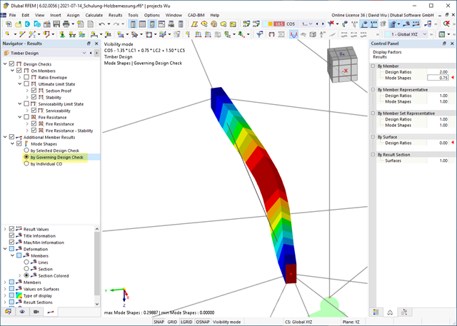
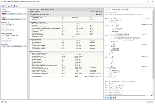
Did you use the eigenvalue solver of the add-on to determine the critical load factor within the stability analysis? If so, you can then display the governing mode shape of the object to be designed as a result. The eigenvalue solver is available here for the lateral-torsional buckling analysis, depending on the design standard used.
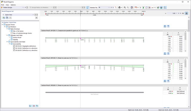
If your design is successful, the relaxed part of your work follows. Because the program does many processes for you. For example, the performed design checks are displayed in a table. It shows you all the result details. Due to the clearly presented design formulas, you will be able to understand the results without any problems. There is no "black box" effect here.
The design checks are carried out at all governing locations of the members and displayed graphically as a result diagram. Furthermore, detailed graphics, such as the stress distribution on a cross-section or the governing mode shape, are available for you in the result output.
All input and result data are part of the RFEM/RSTAB printout report. You can select the report contents and extent specifically for the individual design checks.

The Dlubal structural analysis software does a lot of work for you. The input parameters, which are relevant for the selected standards, are suggested by the program in accordance with the rules. Furthermore, you can enter response spectra manually.
Load cases of the type Response Spectrum Analysis define the direction in which response spectra act and which eigenvalues of the structure are relevant for the analysis. In the spectral analysis settings, you can define details for the combination rules, damping (if applicable), and zero-period acceleration (ZPA).

Did you know that Equivalent static loads are generated separately for each relevant eigenvalue and excitation direction. These loads are saved in a load case of the Response Spectrum Analysis type and RFEM/RSTAB performs a linear static analysis.

The load cases of the type Response Spectrum Analysis contain the generated equivalent loads. First, the modal contributions have to be superimposed with the SRSS or CQC rule. In this case, you can use the signed results based on the dominant mode shape.
Afterwards, the directional components of earthquake actions are combined with the SRSS or the 100% / 30% rule.