81 Wyniki
Wyświetl wyniki:
Sortuj według:
- 002074
- Ogólne informacje
- Analiza stateczności konstrukcji RFEM 6
- Analiza stateczności konstrukcji RSTAB 9
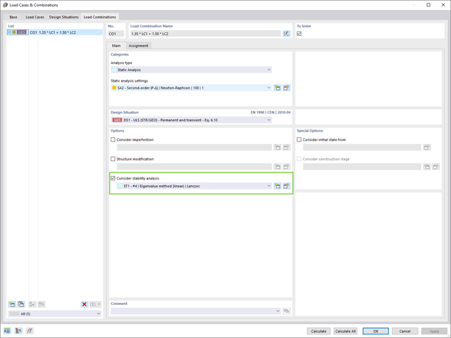
Jeżeli w programie istnieje przypadek obciążenia lub kombinacja obciążeń, obliczenia stateczności są aktywowane. Można zdefiniować inny przypadek obciążenia, na przykład w celu uwzględnienia naprężenia początkowego.
W tym celu należy określić, czy ma zostać przeprowadzona analiza liniowa czy nieliniowa. W zależności od przypadku zastosowania, można wybrać bezpośrednią metodę obliczeniową, taką jak metoda Lanczosa lub metoda iteracji ICG. Pręty niezintegrowane z powierzchniami są zazwyczaj wyświetlane jako elementy prętowe z dwoma węzłami ES. W przypadku zastosowania takich elementów program nie może określić wyboczenia lokalnego pojedynczych prętów. Z tego względu'istnieje możliwość automatycznego dzielenia prętów.
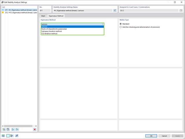
W przypadku analizy wartości własnych dostępnych jest kilka metod:
- Metody bezpośrednie
- Metody bezpośrednie (Lanczosa [RFEM], pierwiastki z wielomianu charakterystycznego [RFEM], metoda iteracji podprzestrzeni [RFEM/RSTAB], przesunięta iteracja odwrócona [RSTAB]) są odpowiednie dla małych i średnich modeli. Z szybkich metod rozwiązywania problemów należy korzystać tylko w przypadku, gdy komputer posiada dużą ilość pamięci RAM.
- Metoda iteracji ICG (niekompletny sprzężony gradient [RFEM])
- Z drugiej strony, ta metoda wymaga tylko niewielkiej ilości pamięci. Wartości własne są określane jedna po drugiej. Może być stosowany do obliczania dużych układów konstrukcyjnych o niewielkiej liczbie wartości własnych.
Rozszerzenie Stateczność konstrukcji umożliwia nieliniową analizę stateczności przy użyciu metody przyrostowej. Analiza ta dostarcza wyniki zbliżone do rzeczywistości również w przypadku konstrukcji nieliniowych. Współczynnik obciążenia krytycznego jest określany poprzez stopniowe zwiększanie obciążeń w podstawowym przypadku obciążenia, aż do osiągnięcia niestateczności. Przyrost obciążenia uwzględnia nieliniowości, takie jak ulegające uszkodzeniu pręty, podpory i fundamenty oraz nieliniowości materiałowe. Po zwiększeniu obciążenia można opcjonalnie przeprowadzić liniową analizę stateczności na ostatnim stabilnym stanie w celu określenia postaci stateczności.
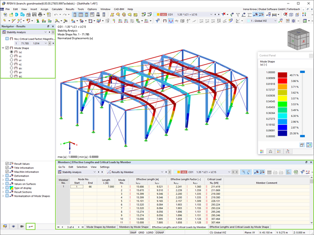
Jako pierwsze wyniki program przedstawia współczynniki obciążenia krytycznego. Następnie można przeprowadzić ocenę zagrożeń stateczności. W przypadku modeli prętowych w tabelach wyświetlane są wynikowe długości efektywne i obciążenia krytyczne prętów.
W następnym oknie wyników można sprawdzić znormalizowane wartości własne posortowane według węzła, pręta i powierzchni. Grafika wartości własnych umożliwia ocenę zachowania wyboczeniowego. Ułatwia to podjęcie środków zaradczych.
- 002073
- Ogólne informacje
- Analiza stateczności konstrukcji RFEM 6
- Analiza stateczności konstrukcji RSTAB 9
- Obliczanie modeli składających się z elementów prętowych, powłokowych i bryłowych
- Nieliniowa analiza stateczności
- Możliwość uwzględniania sił osiowych od wstępnego sprężenia
- Cztery dostępne solvery do rozwiązywania równań dla efektywnego obliczania różnych modeli konstrukcyjnych
- Opcjonalne uwzględnianie zmian w sztywności w programie RFEM/RSTAB
- Wyszukiwanie postaci wyboczeniowych o krytycznym mnożniku obciążenia większym niż zadany przez użytkownika (metoda "przesunięcia")
- Możliwość określania wektorów własnych dla modeli niestatecznych (w celu zidentyfikowania przyczyny niestateczności)
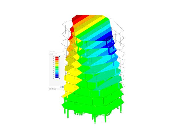
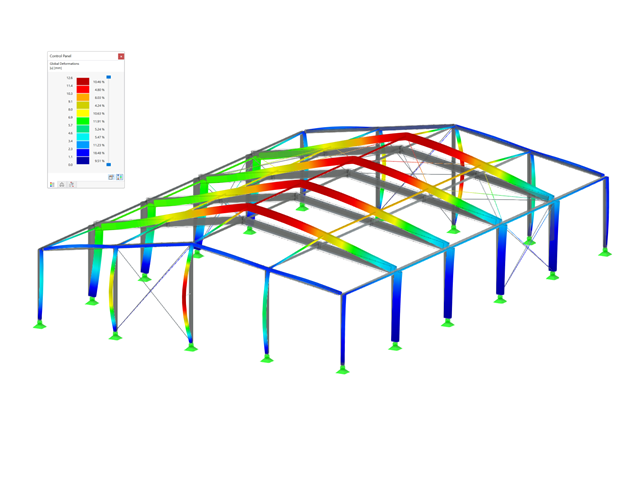
- Wizualizacja postaci niestateczności
- Podstawa określania imperfekcji
- 002089
- Ogólne informacje
- Skręcanie skrępowane (7 stopni swobody) RFEM 6
- Skręcanie skrępowane (7 stopni swobody) RSTAB 9
- Uwzględnienie 7 lokalnych kierunków deformacji (ux , uy, uz, φx, φy, φz, ω ) lub 8 sił wewnętrznych (N , Vu, Vv, Mt, pri, Mt, s, Mu, Mv, Mω ) przy obliczaniu elementów prętowych
- Możliwość stosowania w połączeniu z analizą statyczno-wytrzymałościową według teorii II rzędu, i analiza dużych deformacji (można również uwzględnić imperfekcje)
- W połączeniu z rozszerzeniem Analiza stateczności umożliwia definiowanie współczynników obciążenia krytycznego i kształtów drgań dla problemów stateczności, takich jak wyboczenie skrętne i zwichrzenie
- Uwzględnianie blach czołowych i usztywnień poprzecznych jako sprężystości skrępowanej podczas obliczania przekrojów dwuteowych z automatycznym określaniem i wyświetlaniem graficznym sztywności sprężystości deplanacyjnej
- Graficzne przedstawienie deplanacji przekroju prętów w stanie odkształcenia
- Pełna integracja z RFEM i RSTAB

- 002090
- Ogólne informacje
- Skręcanie skrępowane (7 stopni swobody) RFEM 6
- Skręcanie skrępowane (7 stopni swobody) RSTAB 9
Obliczenia skręcania skrępowanego można przeprowadzić dla całego układu. Uwzględniasz zatem dodatkową wartość 7 stopnia swobody w obliczeniach pręta. Sztywności połączonych elementów konstrukcyjnych są uwzględniane automatycznie. Oznacza to, że nie ma potrzeby' definiowania równoważnych sztywności sprężystych ani warunków podparcia dla układu odłączanego.
Następnie można wykorzystać siły wewnętrzne z obliczeń ze skręcaniem skrępowanym w rozszerzeniu do obliczeń. W zależności od materiału i wybranej normy należy uwzględnić bimoment wyboczeniowy i drugorzędny moment skręcający. Typowym zastosowaniem jest analiza stateczności według teorii drugiego rzędu z wykorzystaniem imperfekcji w konstrukcjach stalowych.
Czy wiecie, że...? Zastosowanie nie ogranicza się do przekrojów stalowych cienkościennych. Pozwala to na przykład na przeprowadzenie obliczeń idealnego momentu krytycznego dla belek o przekrojach z drewna litego.
- 002111
- Ogólne informacje
- Analiza naprężeniowo-odkształceniowa RFEM 6
- Analiza naprężeniowo-odkształceniowa RSTAB 9
- Ogólna analiza naprężeniowa
- Automatyczny import sił wewnętrznych z programu RFEM/RSTAB
- Graficzne i numeryczne przedstawianie naprężeń, odkształceń, luzu i stopni wykorzystania w pełni zintegrowane z RFEM/RSTAB
- Zdefiniowana przez użytkownika specyfikacja naprężenia granicznego
- Podsumowanie podobnych elementów konstrukcyjnych do obliczeń
- Szeroki zakres opcji umożliwiających dostosowywania sposobu wyświetlania wyników
- Przejrzyste tabele wyników dla szybkiego ich przeglądania po zakończeniu obliczeń
- Łatwa możliwość identyfikacji wyników dzięki w pełni udokumentowanej metodzie obliczeniowej wraz ze wszystkimi wzorami
- Wysoka wydajność pracy dzięki minimalnej ilości danych wejściowych
- Elastyczność dzięki szczegółowym opcjom ustawień dla podstawy i zakresu obliczeń
- Wyświetlanie szarej strefy dla nieistotnych zakresów wartości: Funkcja produktu "Analiza naprężeniowo-odkształceniowa z wyświetlaniem w szarej strefie"
- 002112
- Ogólne informacje
- Analiza naprężeniowo-odkształceniowa RFEM 6
- Analiza naprężeniowo-odkształceniowa RSTAB 9
- Optymalizacja przekroju
- Transfer zoptymalizowanych przekrojów do RFEM/RSTAB
- Wymiarowanie dowolnego przekroju cienkościennego z RSECTION
- Odwzorowanie wykresu naprężeń na przekroju
- Wyznaczanie naprężeń normalnych, ścinających i równoważnych
- Wyświetlanie składowych naprężeń dla poszczególnych typów sił wewnętrznych pręta
- Szczegółowe przedstawienie naprężeń we wszystkich punktach naprężeniowych
- Wyznaczanie największego Δσ dla każdego punktu naprężenia (na przykład do obliczeń zmęczenia)
- Wyświetlanie w kolorze naprężeń i stopni wykorzystania w celu szybkiego przeglądu stref krytycznych lub przewymiarowanych
- Wyświetlanie wykazów materiałów
- Wyznaczanie naprężeń głównych i podstawowych, naprężeń membranowych i stycznych oraz naprężeń zastępczych i zastępczych naprężeń membranowych
- Analiza naprężeń dla elementów konstrukcyjnych o dowolnym kształcie
- Obliczanie naprężeń zastępczych według różnych metod:
- Hipoteza energii odkształcenia (von Mises)
- Schubspannungshypothese (Tresca)
- Normalspannungshypothese (Rankine)
- Hauptdehnungshypothese (Bach)
- Możliwość optymalizacji grubości powierzchni i transferu danych do programu RFEM
- Ausgabe der Dehnungen
- Szczegółowe wyniki dla różnych składników naprężeń i stopni wykorzystania w tabelach i w grafice
- Filtermöglichkeit für Volumenkörper, Flächen, Linien und Knoten in Tabellen
- Querschubspannungen nach Mindlin, Kirchhoff oder freier Eingabe
- Spannungsauswertung für Schweißnähte an Verbindungslinien zwischen Flächen: Przejdź do funkcji produktu "Spoina liniowa"
- 002115
- Wyniki
- Analiza naprężeniowo-odkształceniowa RFEM 6
- Analiza naprężeniowo-odkształceniowa RSTAB 9
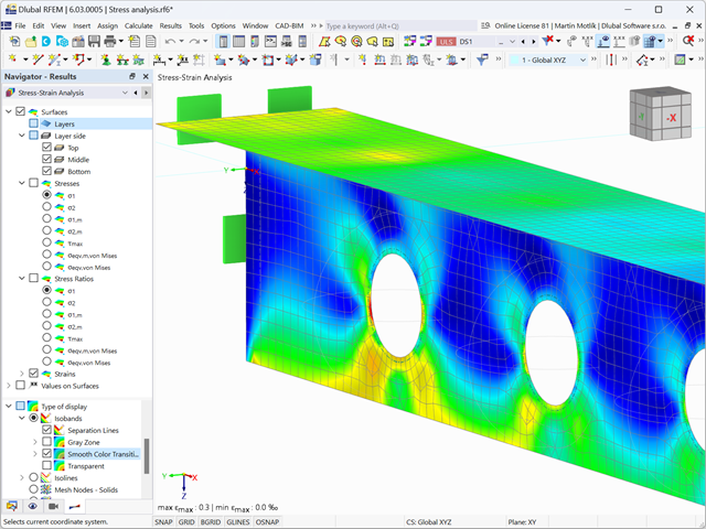
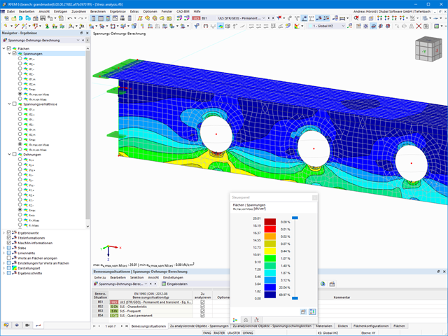
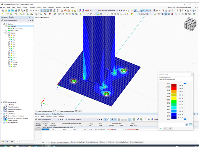
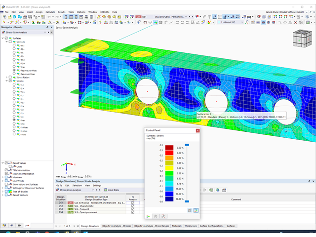
Po zakończeniu obliczeń wyniki są uporządkowane w sposób przejrzysty. W ten sposób program wyświetla maksymalne naprężenia i stopnie naprężeń posortowane według przekroju, pręta/powierzchni, bryły, zbioru prętów, położenia x itd. Oprócz wartości wyników w formie tabelarycznej rozszerzenie wyświetla również odpowiednią grafikę przekroju z punktami naprężeniowymi, wykresem naprężeń i wartościami. Stopień wykorzystania można odnieść do dowolnego rodzaju naprężenia. Aktualnie wybrana lokalizacja na elemencie zostanie wyróżniona na modelu analitycznym w programie RFEM/RSTAB.
Oprócz oceny tabelarycznej program oferuje jeszcze więcej. Naprężenia i stopnie wykorzystania można również sprawdzić graficznie na modelu w programie RFEM/RSTAB. Istnieje możliwość indywidualnego dostosowania kolorów i wartości.
Wyświetlanie wykresów wyników dla pręta lub zbioru prętów umożliwia dokładną ocenę. Dla każdego miejsca obliczeniowego można otworzyć odpowiednie okno dialogowe, w którym można sprawdzić odpowiednie do obliczeń właściwości przekroju i składowe naprężeń w dowolnym punkcie naprężeniowym. Na koniec istnieje możliwość wydrukowania odpowiedniej grafiki wraz ze wszystkimi szczegółami obliczeń.
- 002401
- Ogólne informacje
- Skręcanie skrępowane (7 stopni swobody) RFEM 6
- Skręcanie skrępowane (7 stopni swobody) RSTAB 9
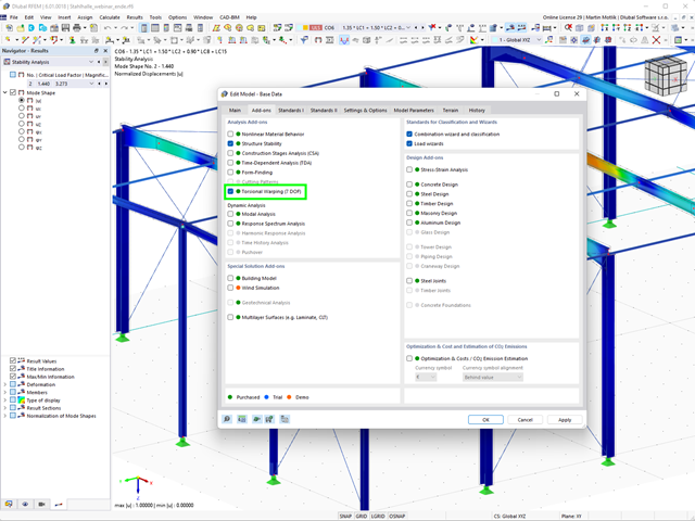
- Funkcję skręcania skrępowanego można aktywować lub dezaktywować w zakładce Rozszerzenia w Danych podstawowych modelu.
- Po aktywowaniu rozszerzenia interfejs użytkownika w programie RFEM zostaje rozszerzony o nowe wpisy w nawigatorze, tabelach i oknach dialogowych.
- 002140
- Ogólne informacje
- Projektowanie konstrukcji aluminiowych RFEM 6
- Projektowanie konstrukcji aluminiowych RSTAB 9
- Szeroki wybór dostępnych przekrojów, takich jak dwuteowniki walcowane; ceowniki; teowniki; kątowniki; profile zamknięte prostokątne i okrągłe; pręty okrągłe; przekroje symetryczne i niesymetryczne, parametryczne przekroje dwuteowe, teowe, kątowniki; przekroje złożone (przydatność do obliczeń zależy od wybranej normy)
- Wymiarowanie ogólnych przekrojów RSECTION (w zależności od formatów obliczeniowych dostępnych w odpowiedniej normie); na przykład obliczanie naprężeń zastępczych
- Wymiarowanie prętów o zbieżnym przekroju (metoda zależna od normy)
- Możliwe jest dostosowanie istotnych współczynników obliczeniowych i parametrów normowych
- Elastyczność dzięki szczegółowym opcjom ustawień dla podstawy i zakresu obliczeń
- Szybkie i przejrzyste wyświetlanie wyników dla globalnej oceny ich rozkładu na konstrukcji po zakończeniu obliczeń
- Szczegółowe wyniki obliczeń i niezbędne wzory (jasna i łatwa do zweryfikowania ścieżka wyników)
- Przejrzyste zestawienie wyników w formie numerycznej w stosownych oknach oraz możliwość ich graficznego przedstawienia na konstrukcji
- Integracja wyników z protokołem wydruku programu RFEM/RSTAB
- 002141
- Ogólne informacje
- Projektowanie konstrukcji aluminiowych RFEM 6
- Projektowanie konstrukcji aluminiowych RSTAB 9
- Wymiarowanie elementów rozciąganych, ściskanych, zginanych, ścinanych, skręcanych i poddanych połączonemu działaniu tych sił wewnętrznych
- Obliczanie rozciągania z uwzględnieniem zredukowanej powierzchni przekroju (np. osłabienie z uwagi na otwory)
- Automatyczna klasyfikacja przekrojów w celu sprawdzenia wyboczenia lokalnego
- Siły wewnętrzne z obliczeń ze skręcaniem skrępowanym (7 stopni swobody) są uwzględniane w kontroli naprężeń zastępczych (obecnie nie dla normy ADM 2020)
- Wymiarowanie przekrojów klasy 4 o właściwościach przekroju efektywnego zgodnie z EN 1999-1-1 (dla przekrojów RSECTION wymagane są licencje dla przekrojów RSECTION i "Przekroje efektywne")
- Sprawdzenie wyboczenia przy ścinaniu z uwzględnieniem usztywnień poprzecznych
- 002142
- Wyniki
- Projektowanie konstrukcji aluminiowych RFEM 6
- Projektowanie konstrukcji aluminiowych RSTAB 9
- Analiza stateczności dla wyboczenia giętnego, wyboczenia skrętnego i wyboczenia giętno-skrętnego przy ściskaniu
- Analiza zwichrzenia elementów poddanych obciążeniu momentem
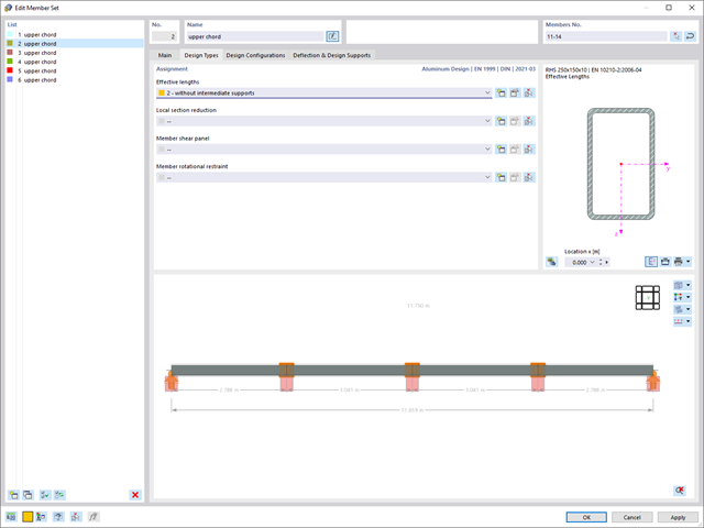
- Import długości efektywnych z obliczeń przy użyciu rozszerzenia Stateczność konstrukcji
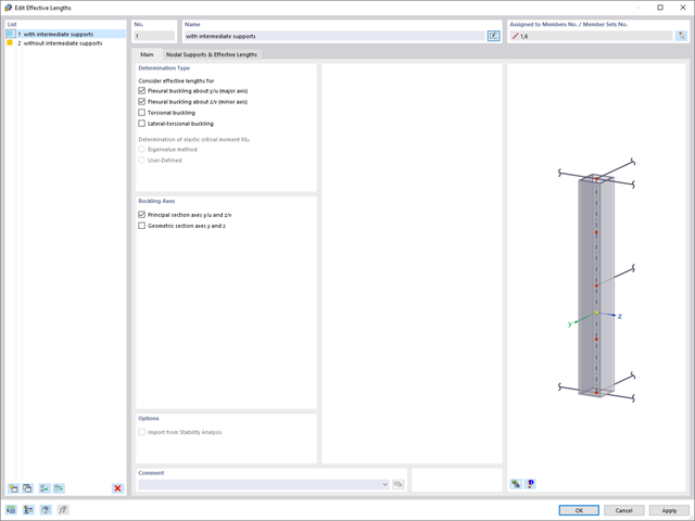
- Graficzne wprowadzanie i kontrola zdefiniowanych podpór węzłowych oraz długości efektywnych w celu analizy stateczności
- W zależności od normy istnieje wybór między wprowadzaniem wartości Mcr przez użytkownika, metodą analityczną z normy lub wykorzystaniem wewnętrznego solwera wartości własnych
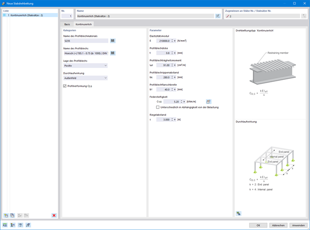
- Uwzględnienie panelu usztywniającego i ograniczenia obrotu podczas korzystania z solwera wartości własnych
- Graficzne przedstawienie postaci własnej w przypadku zastosowania solwera wartości własnych
- Analiza stateczności elementów konstrukcyjnych ze ściskaniem i naprężeniem zginającym, w zależności od normy obliczeniowej
- Przejrzyste obliczanie wszystkich niezbędnych współczynników, takich jak współczynniki interakcji
- Alternatywne uwzględnienie wszystkich wpływów dla analizy stateczności podczas określania sił wewnętrznych w programie RFEM/RSTAB (analiza drugiego rzędu, imperfekcje, redukcja sztywności, ewentualnie w połączeniu z rozszerzeniem Skręcanie skrępowane (7 stopni swobody))
- Automatyczne uwzględnianie masy własnej od ciężaru konstrukcji
- Możliwy bezpośredni import mas z przypadków obciążeń lub kombinacji
- Opcjonalne definiowanie mas dodatkowych (masy węzłowe, liniowe lub powierzchniowe oraz masy wynikające z bezwładności) bezpośrednio w przypadkach obciążeń
- Opcjonalne pominięcie mas (na przykład masy fundamentów)
- Kombinacje mas w różnych przypadkach i kombinacjach obciążeń
- Predefiniowane współczynniki kombinacji wg różnych norm (EC 8, SIA 261, ASCE 7, ...)
- Opcjonalny import stanów początkowych (np. w celu uwzględnienia naprężenia wstępnego i imperfekcji)
- modyfikacja konstrukcji
- Uwzględnianie uszkodzenia w podporach lub prętach/powierzchniach/bryłach
- Możliwość zadania kilku analiz modalnych (np. w celu analizy różnych mas lub modyfikacji sztywności)
- Wybór typu macierzy mas (macierz diagonalna, macierz spójna, macierz jednostkowa) oraz wskazanych przez użytkownika stopni swobody (translacyjne i rotacyjne)
- Metody określania liczby postaci drgań własnych (liczba zdefiniowana przez użytkownika, liczba określana automatycznie - w celu osiągnięcia zadanych efektywnych współczynników masy modalnej, liczba określana automatycznie - w celu osiągnięcia maksymalnej częstotliwości drgań własnych - dostępne tylko w programie RSTAB)
- Określanie postaci drgań i mas w węzłach siatki MES
- Wyniki w postaci wartości własnych, częstości kątowych, częstotliwości drgań własnych i okresu drgań własnych
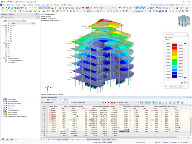
- Wyniki w postaci mas modalnych, efektywnych mas modalnych, współczynników masy modalnej i współczynników udziału masy
- Tabelaryczne i graficzne przedstawienie mas w punktach siatki MES
- Wizualizacja i animacja postaci drgań własnych
- Różne opcje skalowania postaci drgań własnych
- Dokumentacja wyników numerycznych i graficznych w raporcie
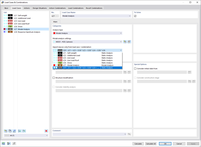
W ustawieniach analizy modalnej należy wprowadzić wszystkie dane, które są niezbędne do określenia częstotliwości drgań własnych. Są to na przykład kształty mas i solwery wartości własnych.
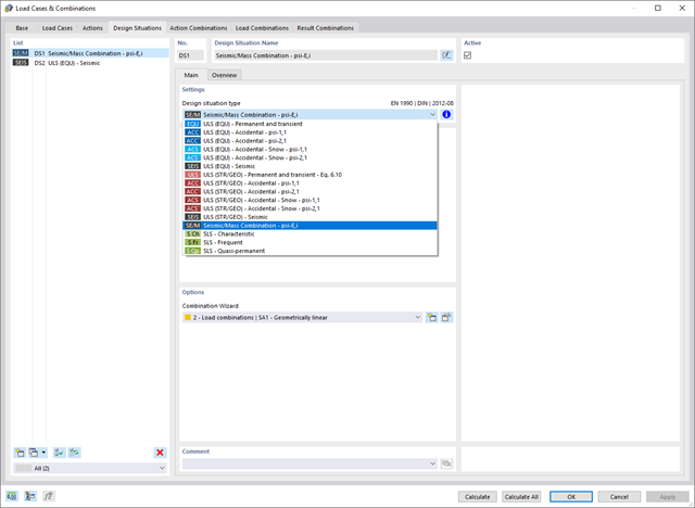
Rozszerzenie Analiza modalna określa najniższe wartości częstości drgań własnych konstrukcji. Liczbę wartości własnych można dostosować lub określić automatycznie. Należy zatem osiągnąć efektywne współczynniki masy modalnej lub maksymalne częstotliwości drgań własnych. Masy są importowane bezpośrednio z przypadków obciążeń i kombinacji obciążeń. W takim przypadku istnieje możliwość uwzględnienia masy całkowitej, składowych obciążenia w globalnym kierunku Z lub tylko składowej obciążenia w kierunku siły ciężkości.
Dodatkowe masy w węzłach, liniach, prętach lub powierzchniach można zdefiniować ręcznie. Ponadto można wpływać na macierz sztywności poprzez import sił osiowych lub modyfikacji sztywności z przypadku obciążenia lub kombinacji obciążeń.
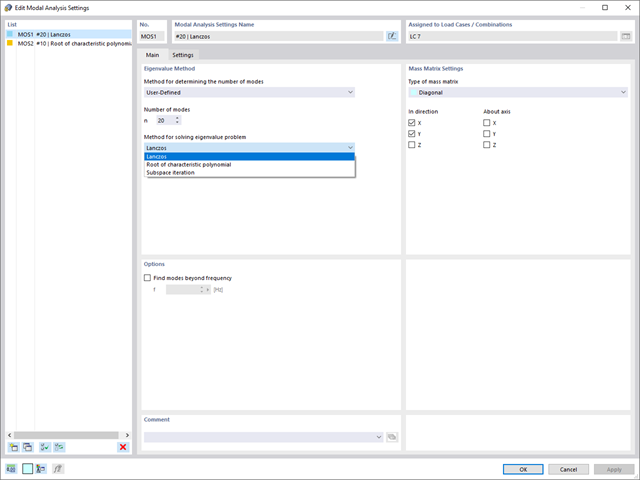
W programie RFEM dostępne są trzy wydajne solwery wartości własnych:
- pierwiastek wielomianu charakterystycznego
- Metoda Lanchosa
- iteracja podprzestrzeni
Z kolei program RSTAB oferuje dwa solwery wartości własnych:
- iteracja podprzestrzeni
- Metoda Powera z przesuniętą odwrotnością
Wybór solwera wartości własnych zależy przede wszystkim od rozmiaru modelu.
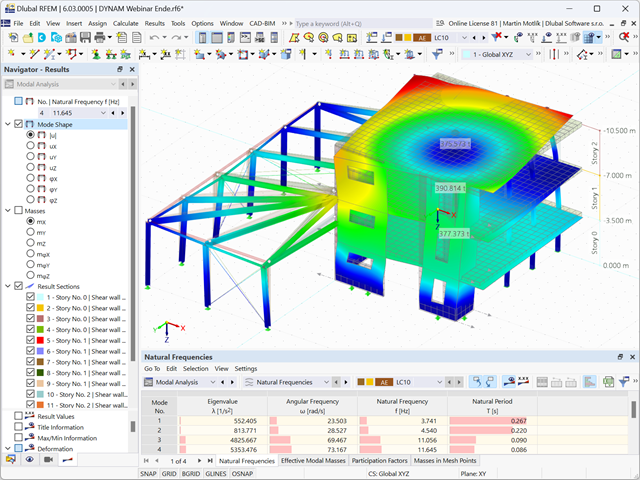
Zaraz po zakończeniu obliczeń wyświetlane są wartości własne, częstotliwości drgań własnych i okresy. Okna z tymi wynikami zintegrowane są z programem głównym RFEM/RSTAB. W tabelach można znaleźć wszystkie kształty drgań konstrukcji, a także można je wyświetlić graficznie i animować.
Wszystkie tabele wyników i grafiki stanowią część raportu programu RFEM/RSTAB. Zapewnia to przejrzystą dokumentację obliczeń. Tabele można również eksportować do programu MS Excel.
- 002162
- Ogólne informacje
- Analiza stateczności konstrukcji RFEM 6
- Analiza stateczności konstrukcji RSTAB 9
W porównaniu z modułami dodatkowymi RF-STABILITY (RFEM 5) i RSBUCK (RSTAB 8) do rozszerzenia Stateczność konstrukcji dla programu RFEM 6/RSTAB 9 dodano następujące nowe funkcje:
- Aktivierung als Eigenschaft eines Lastfalls oder einer Lastkombination
- Automatisierte Aktivierung der Stabilitätsberechnung über Kombinationsassistenten für mehrere Lastsituationen in einem Schritt
- Inkrementelle Laststeigerung mit benutzerdefinierten Abbruchkriterien
- Veränderung der Eigenformnormierung ohne Neuberechnung
- Ergebnistabellen mit Filteroption
- 002165
- Ogólne informacje
- Skręcanie skrępowane (7 stopni swobody) RFEM 6
- Skręcanie skrępowane (7 stopni swobody) RSTAB 9
W porównaniu z modułem dodatkowym RF-/STEEL Warping Torsion (RFEM 5/RSTAB 8) do rozszerzenia Skręcanie skrępowane (7 DOF) dla programu RFEM 6/RSTAB 9 dodano następujące nowe funkcje:
- Pełna integracja ze środowiskiem RFEM 6 i RSTAB 9
- Siódmy stopień swobody jest bezpośrednio uwzględniany w obliczeniach prętów w programie RFEM/RSTAB na całym układzie
- Nie ma już potrzeby definiowania warunków podparcia lub sztywności sprężystej do obliczeń w uproszczonym układzie zastępczym
- Możliwość łączenia z innymi rozszerzeniami, na przykład do obliczania obciążeń krytycznych dla wyboczenia skrętnego i zwichrzenia z analizą stateczności
- Brak ograniczeń dla stalowych przekrojów cienkościennych (możliwe jest również obliczenie momentu krytycznego, na przykład dla belek o masywnych przekrojach drewnianych)
W porównaniu z modułem dodatkowym RF-/DYNAM Pro-Natural Vibrations (RFEM 5/RSTAB 8) do rozszerzenia Analiza modalna dla programu RFEM 6/RSTAB 9 dodano następujące nowe funkcje:
- Predefiniowane współczynniki kombinacji dla różnych norm (EC 8, ASCE itp.)
- Opcjonalne pominięcie mas (na przykład masy fundamentów)
- Metody określania liczby postaci drgań własnych (liczba zdefiniowana przez użytkownika, liczba określana automatycznie - w celu osiągnięcia zadanych efektywnych współczynników masy modalnej, liczba określana automatycznie - w celu osiągnięcia maksymalnej częstotliwości drgań własnych)
- Wyniki w postaci mas modalnych, efektywnych mas modalnych, współczynników masy modalnej i współczynników udziału masy
- Tabelaryczne i graficzne przedstawienie mas w punktach siatki MES
- Różne opcje skalowania postaci drgań własnych w nawigatorze wyników
- 002169
- Ogólne informacje
- Analiza naprężeniowo-odkształceniowa RFEM 6
- Analiza naprężeniowo-odkształceniowa RSTAB 9
W porównaniu z modułem dodatkowym RF-/STEEL (RFEM 5/RSTAB 8) do rozszerzenia Analiza naprężeniowo-odkształceniowa dla programu RFEM 6/RSTAB 9 dodano następujące nowe funkcje:
- Możliwość analizy prętów, powierzchni, brył, spoin (połączenia spawane liniowo między dwiema i trzema powierzchniami z późniejszym obliczaniem naprężeń)
- Wyświetlanie naprężeń, stopni naprężeń, zakresów naprężeń i odkształceń
- Naprężenie graniczne w zależności od przydzielonego materiału lub danych wejściowych zdefiniowanych przez użytkownika
- Indywidualne określenie wyników do obliczeń poprzez dowolnie przydzielane typów ustawień
- Szczegóły dla wyników niemodalnych z wyświetlaniem przygotowanego wzoru i dodatkowym wyświetlaniem wyników na poziomie przekroju prętów
- Możliwość wygenerowania zastosowanych wzorów do kontroli obliczeń
- 002173
- Ogólne informacje
- Projektowanie konstrukcji aluminiowych RFEM 6
- Projektowanie konstrukcji aluminiowych RSTAB 9
W porównaniu z modułem dodatkowym RF-/ALUMINIUM (RFEM 5/RSTAB 8) do rozszerzenia Projektowanie konstrukcji aluminiowych dla programu RFEM 6/RSTAB 9 dodano następujące nowe funkcje:
- Oprócz Eurokodu 9, dostępna jest amerykańska norma ADM 2020.
- Uwzględnienie stabilizującego efektu płatwi i blachy trapezowej za pomocą podparcia obrotowych stopni swobody oraz paneli usztywniających
- Graficzne przedstawienie wyników na przekroju brutto
- Wyświetlanie odpowiednich wzorów użytych do sprawdzania warunków nośności (w tym odniesienie do zastosowanego równania z normy)
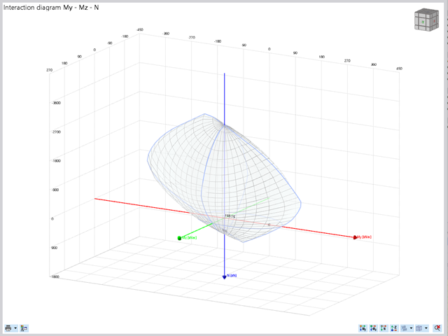
Projektowanie konstrukcji betonowych | Wykres interakcji My-Mz-N (3D) przekrojów z betonu zbrojonego
Na pytanie 'Ile można przewozić?' zazwyczaj odpowiada 'Tak'. Do graficznego przedstawiania stanu granicznego nośności przekrojów żelbetowych wymagany jest trójwymiarowy wykres interakcji momentu-momentu-siła osiowa. Oprogramowanie do analizy statyczno-wytrzymałościowej firmy Dlubal właśnie to oferuje.
Dzięki dodatkowemu wyświetleniu oddziaływania obciążenia można łatwo rozpoznać lub zwizualizować przekroczenie granicznej nośności przekroju żelbetowego. Ponieważ możesz kontrolować właściwości wykresu, możesz dostosować wygląd wykresu My-Mz-N do swoich potrzeb.
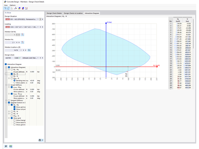
Czy wiesz, że wykresy interakcji moment-siła (wykresy MN) można wyświetlić również graficznie? Umożliwia to wyświetlenie nośności przekroju w przypadku interakcji momentu zginającego i siły osiowej. Oprócz wykresów interakcji związanych z osiami przekroju (wykres My-N i wykres Mz-N) można również wygenerować indywidualny wektor momentów w celu utworzenia wykresu interakcji Mres -N. Płaszczyznę przekroju wykresów MN można wyświetlić na wykresie interakcji 3D.Program wyświetla odpowiednie pary wartości stanu granicznego nośności w tabeli. Tabela jest dynamicznie powiązana z wykresem, dzięki czemu wybrany punkt graniczny jest również wyświetlany na wykresie.
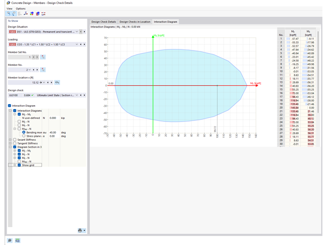
Czy chcesz określić nośność przekroju żelbetowego na zginanie dwukierunkowe? W tym celu należy najpierw aktywować wykres interakcji moment-moment (wykres My-Mz). Wykres My-Mz przedstawia poziomy przekrój przez trójwymiarowy wykres dla określonej siły osiowej N. Dzięki połączeniu z trójwymiarowym wykresem interakcji można tam również zwizualizować płaszczyznę przekroju.
.png?mw=640&hash=5a991f211d984ac624978f514e70c53da263e5d9)
W zależności od siły osiowej N, można wygenerować linię krzywizny momentu dla dowolnego wektora momentu. Program pokazuje również pary wartości wyświetlanego wykresu w tabeli. Ponadto można aktywować jako dodatkowy wykres sieczny i sztywność styczną przekroju żelbetowego, należące do wykresu krzywizny momentu.
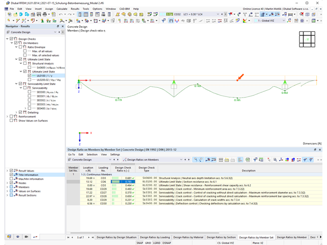
Program do analizy statyczno-wytrzymałościowej zapewnia przejrzysty przegląd wszystkich przeprowadzonych kontroli obliczeń dla określonej normy obliczeniowej. Dla każdego warunku projektowego należy określić kryterium obliczeniowe. Oprócz sprawdzania stanu granicznego nośności i użytkowalności program sprawdza zasady projektowania określone w normie. Dla każdej kontroli obliczeń są określone szczegóły obliczeń, w tym wartości początkowe, wyniki pośrednie i wyniki końcowe. Proces obliczeń wraz z zastosowanymi wzorami, standardowymi źródłami i wynikami szczegółowo przedstawiony jest w oknie informacyjnym w szczegółach obliczeń.
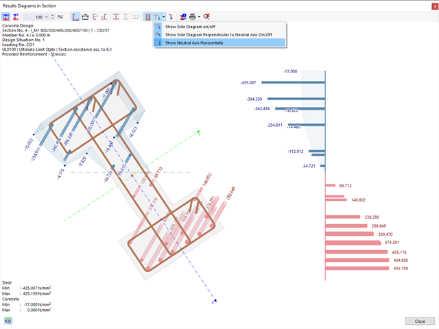
Istniejące naprężenia i odkształcenia przekroju betonowego i zbrojenia można wyświetlić w postaci obrazu naprężeń 3D lub grafiki 2D. W zależności od tego, które wyniki zostaną wybrane w drzewie wyników, naprężenia lub odkształcenia są wyświetlane w zdefiniowanym zbrojeniu podłużnym pod oddziaływaniami obciążeń lub granicznymi siłami wewnętrznymi.
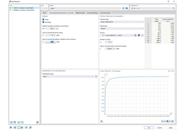
Właściwości betonu, zależne od czasu, takie jak pełzanie i skurcz, są bardzo ważne dla obliczeń. Można je zdefiniować bezpośrednio dla materiału w programie do analizy statyczno-wytrzymałościowej. W oknie dialogowym do wprowadzania danych wyświetlany jest przebieg czasowy funkcji pełzania lub skurczu. Można łatwo wybrać modyfikację zastosowanego wieku betonu, na przykład ze względu na obróbkę termiczną.