88 Wyniki
Wyświetl wyniki:
Sortuj według:
- 002140
- Ogólne informacje
- Projektowanie konstrukcji aluminiowych RFEM 6
- Projektowanie konstrukcji aluminiowych RSTAB 9
- Szeroki wybór dostępnych przekrojów, takich jak dwuteowniki walcowane; ceowniki; teowniki; kątowniki; profile zamknięte prostokątne i okrągłe; pręty okrągłe; przekroje symetryczne i niesymetryczne, parametryczne przekroje dwuteowe, teowe, kątowniki; przekroje złożone (przydatność do obliczeń zależy od wybranej normy)
- Wymiarowanie ogólnych przekrojów RSECTION (w zależności od formatów obliczeniowych dostępnych w odpowiedniej normie); na przykład obliczanie naprężeń zastępczych
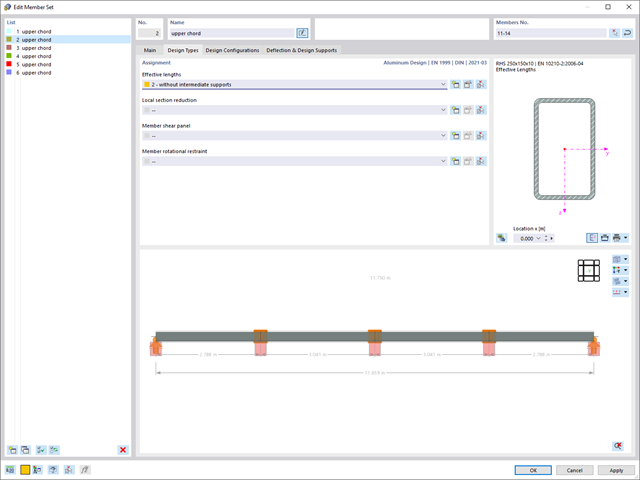
- Wymiarowanie prętów o zbieżnym przekroju (metoda zależna od normy)
- Możliwe jest dostosowanie istotnych współczynników obliczeniowych i parametrów normowych
- Elastyczność dzięki szczegółowym opcjom ustawień dla podstawy i zakresu obliczeń
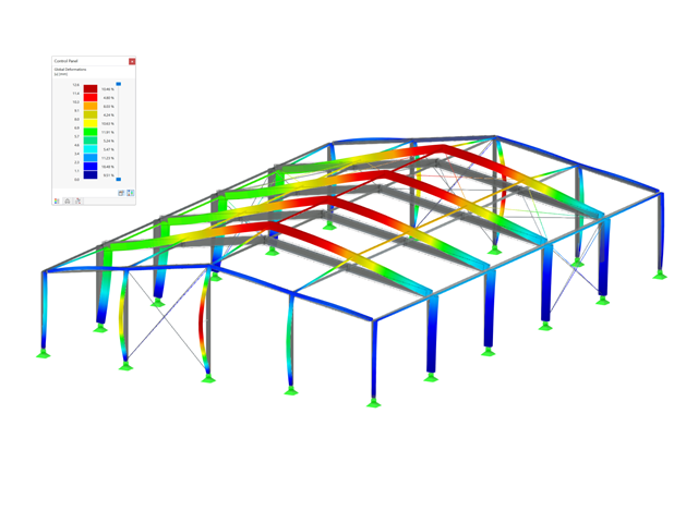
- Szybkie i przejrzyste wyświetlanie wyników dla globalnej oceny ich rozkładu na konstrukcji po zakończeniu obliczeń
- Szczegółowe wyniki obliczeń i niezbędne wzory (jasna i łatwa do zweryfikowania ścieżka wyników)
- Przejrzyste zestawienie wyników w formie numerycznej w stosownych oknach oraz możliwość ich graficznego przedstawienia na konstrukcji
- Integracja wyników z protokołem wydruku programu RFEM/RSTAB
- 002141
- Ogólne informacje
- Projektowanie konstrukcji aluminiowych RFEM 6
- Projektowanie konstrukcji aluminiowych RSTAB 9
- Wymiarowanie elementów rozciąganych, ściskanych, zginanych, ścinanych, skręcanych i poddanych połączonemu działaniu tych sił wewnętrznych
- Obliczanie rozciągania z uwzględnieniem zredukowanej powierzchni przekroju (np. osłabienie z uwagi na otwory)
- Automatyczna klasyfikacja przekrojów w celu sprawdzenia wyboczenia lokalnego
- Siły wewnętrzne z obliczeń ze skręcaniem skrępowanym (7 stopni swobody) są uwzględniane w kontroli naprężeń zastępczych (obecnie nie dla normy ADM 2020)
- Wymiarowanie przekrojów klasy 4 o właściwościach przekroju efektywnego zgodnie z EN 1999-1-1 (dla przekrojów RSECTION wymagane są licencje dla przekrojów RSECTION i "Przekroje efektywne")
- Sprawdzenie wyboczenia przy ścinaniu z uwzględnieniem usztywnień poprzecznych
- 002142
- Wyniki
- Projektowanie konstrukcji aluminiowych RFEM 6
- Projektowanie konstrukcji aluminiowych RSTAB 9
- Analiza stateczności dla wyboczenia giętnego, wyboczenia skrętnego i wyboczenia giętno-skrętnego przy ściskaniu
- Analiza zwichrzenia elementów poddanych obciążeniu momentem
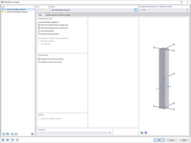
- Import długości efektywnych z obliczeń przy użyciu rozszerzenia Stateczność konstrukcji
- Graficzne wprowadzanie i kontrola zdefiniowanych podpór węzłowych oraz długości efektywnych w celu analizy stateczności
- W zależności od normy istnieje wybór między wprowadzaniem wartości Mcr przez użytkownika, metodą analityczną z normy lub wykorzystaniem wewnętrznego solwera wartości własnych
- Uwzględnienie panelu usztywniającego i ograniczenia obrotu podczas korzystania z solwera wartości własnych
- Graficzne przedstawienie postaci własnej w przypadku zastosowania solwera wartości własnych
- Analiza stateczności elementów konstrukcyjnych ze ściskaniem i naprężeniem zginającym, w zależności od normy obliczeniowej
- Przejrzyste obliczanie wszystkich niezbędnych współczynników, takich jak współczynniki interakcji
- Alternatywne uwzględnienie wszystkich wpływów dla analizy stateczności podczas określania sił wewnętrznych w programie RFEM/RSTAB (analiza drugiego rzędu, imperfekcje, redukcja sztywności, ewentualnie w połączeniu z rozszerzeniem Skręcanie skrępowane (7 stopni swobody))
Parametry załączników krajowych (NA) do Eurokodu 3 z następujących krajów są zintegrowane:
-
 DIN EN 1993-1-1/NA:2016-04 (Niemcy)
 -
 ÖNORM EN 1993-1-1/NA:2015-12 (Austria)
 -
 SN EN 1993-1-1/NA:2016-07 (Szwajcaria)
 -
 BDS EN 1993-1-1/NA:2015-10 (Bułgaria)
 -
 BS EN 1993-1-1/NA:2016-07 (Wielka Brytania)
 -
 CEN EN 1993-1-1/2015-06 (Unia Europejska)
 -
 CYS EN 1993-1-1/NA:2015-07 (Cypr)
 -
 CSN EN 1993-1-1/NA:2016-06 (Republika Czeska)
 -
 DS EN 1993-1-1/NA:2015-07 (Dania)
 -
 ELOT EN 1993-1-1/NA:2017-01 (Grecja)
 -
 EVS EN 1993-1-1/NA:2015-08 (Estonia)
 -
 HRN EN 1993-1-1/NA:2016-03 (Chorwacja)
 -
 I S. EN 1993-1-1/NA:2016-03 (Irlandia)
 -
 ILNAS EN 1993-1-1/NA:2015-06 (Luksemburg)
 -
 IST EN 1993-1-1/NA:2015-11 (Islandia)
 -
 LST EN 1993-1-1/NA:2017-01 (Litwa)
 -
 LVS EN 1993-1-1/NA:2015-10 (Łotwa)
 -
 MS EN 1993-1-1/NA:2010-01 (Malezja)
 -
 MSZ EN 1993-1-1/NA:2015-11 (Węgry)
 -
 NBN EN 1993-1-1/NA:2015-07 (Belgia)
 -
 NEN EN 1993-1-1/NA:2016-12 (Holandia)
 -
 NF EN 1993-1-1/NA:2016-02 (Francja)
 -
 NP EN 1993-1-1/NA:2009-03 (Portugalia)
 -
 NS EN 1993-1-1/NA:2015-09 (Norwegia)
 -
 PN EN 1993-1-1/NA:2015-08 (Polska)
 -
 SFS EN 1993-1-1/NA:2015-08 (Finlandia)
 -
 SIST EN 1993-1-1/NA:2016-09 (Słowenia)
 -
 SR EN 1993-1-1/NA:2016-04 (Rumunia)
 -
 SS EN 1993-1-1/NA:2019-05 (Singapur)
 -
 SS EN 1993-1-1/NA:2015-06 (Szwecja)
 -
 STN EN 1993-1-1/NA:2015-10 (Słowacja)
 -
 TKP EN 1993-1-1/NA:2015-04 (Białoruś)
 -
 UNE EN 1993-1-1/NA:2016-02 (Hiszpania)
 -
 UNI EN 1993-1-1/NA:2015-08 (Włochy)
- Proste definiowanie etapów budowy konstrukcji w RFEM wraz z wizualizacją
- Dodawanie, usuwanie, modyfikowanie i reaktywacja elementów prętowych, powierzchniowych i bryłowych oraz ich właściwości (np. przeguby prętowe i liniowe, stopnie swobody dla podpór itp.)
- Ręczna oraz automatyczna kombinatoryka obciążeń na poszczególnych etapach budowy konstrukcji (np. w celu uwzględnienia obciążeń montażowych, tymczasowych urządzeń dźwigowych itp.)
- Uwzględnienie wpływów nieliniowych, takich jak uszkodzenie prętów rozciąganych lub nieliniowe zachowanie podpór
- Interakcja z innymi rozszerzeniami, takimi jak z. B. Nieliniowe zachowanie materiału, Stateczność konstrukcji, -rstab-9/additional-analyses/form-finding/form-finding itd.
- Wyświetlanie wyników w postaci numerycznej i graficznej dla poszczególnych etapów budowy
- Szczegółowy protokół wydruku wraz z dokumentacją wszystkich danych konstrukcyjnych i obciążeń dla każdego etapu budowy
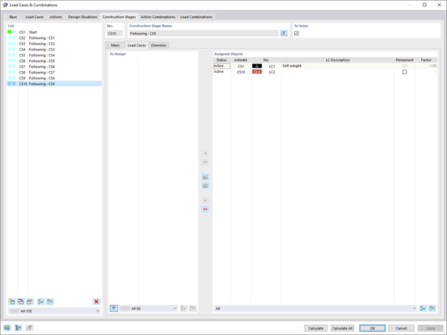
Czy udało Ci się utworzyć całą konstrukcję w programie RFEM? Dobrze, teraz można przypisać poszczególne elementy konstrukcyjne i przypadki obciążeń do odpowiednich etapów budowy. Na każdym etapie budowy można modyfikować na przykład definicje zwolnień prętów i podpór.
Pozwala to na modelowanie zmian konstrukcyjnych, na przykład podczas betonowania dźwigarów mostowych lub osiadania słupów. Przypadki obciążeń utworzone w programie RFEM należy następnie przydzielić do etapów budowy jako obciążenia stałe lub przejściowe.
Czy wiecie, że...? Kombinatoryka umożliwia nakładanie obciążeń stałych i przejściowych w kombinacjach obciążeń. W ten sposób można określić maksymalne siły wewnętrzne dla różnych pozycji dźwigu lub uwzględnić tymczasowe obciążenia montażowe dostępne tylko w jednym etapie budowy.
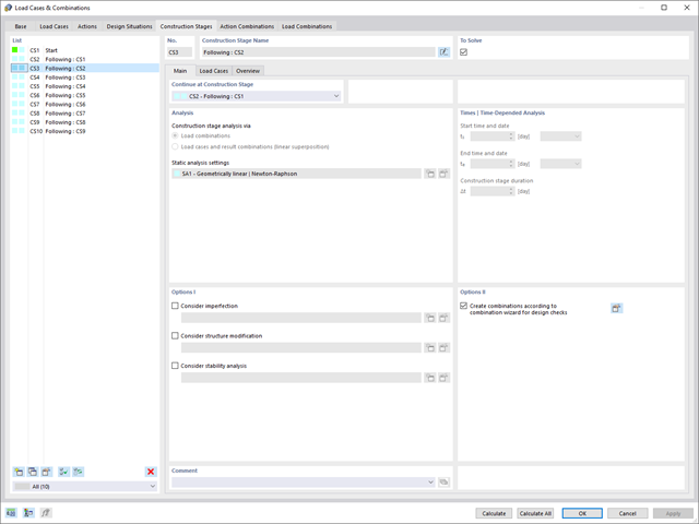
Jeżeli między idealnym układem a układem, który uległ deformacji z poprzedniego etapu budowy, pojawią się różnice w geometrii, są one porównywane w programie. Następujące po sobie kolejne etapy budowy obliczane są na bazie układu konstrukcyjnego z odkształceniami i obciążeniami wynikającymi z poprzednich etapu budowy. Obliczenia te są nieliniowe.
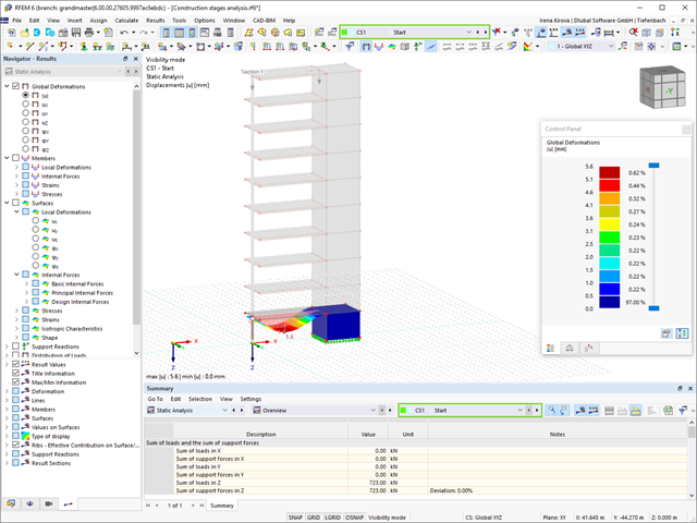
Czy obliczenia zakończyły się pomyślnie? Wyniki poszczególnych etapów budowy można teraz wyświetlać graficznie oraz w tabelach w programie RFEM. Ponadto program RFEM umożliwia uwzględnienie etapów budowy w kombinatoryce i uwzględnienie ich w dalszych obliczeniach.
_(1).png?mw=640&hash=415f7bbaf70e41679bb0106e1cf91eaa8c493ec9)
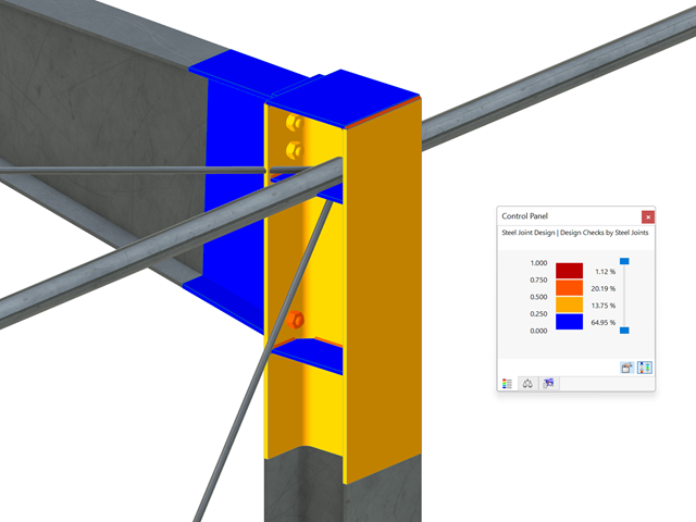
- Automatyczne generowanie modeli do analizy ES: rozszerzenie automatycznie tworzy w tle model elementów skończonych (ES) połączenia stalowego.
- Uwzględnienie wszystkich sił wewnętrznych: Obliczenia obejmują wszystkie siły wewnętrzne (N , Vy, Vz ,My, Mz, MT ) i nie są ograniczone do obciążeń płaskich.
- Automatyczne przenoszenie obciążeń: Wszystkie kombinacje obciążeń są automatycznie przenoszone do modelu analitycznego ES połączenia. Obciążenia są przenoszone bezpośrednio z programu RFEM, dzięki czemu ręczne wprowadzanie danych nie jest konieczne.
- Wydajne modelowanie: Rozszerzenie pozwala zaoszczędzić czas podczas modelowania złożonych sytuacji związanych z połączeniami. Utworzony model analityczny ES można również zapisać i wykorzystać do własnych szczegółowych analiz.
- Rozszerzalna biblioteka: Dostępna jest obszerna, rozszerzalna biblioteka zawierająca wstępnie zdefiniowane szablony połączeń stalowych.
- Szerokie zastosowanie: Rozszerzenie jest odpowiednie do tworzenia połączeń każdego typu i kształtu, jest kompatybilne z prawie wszystkimi przekrojami walcowanymi, spawanymi, złożonymi i cienkościennymi.
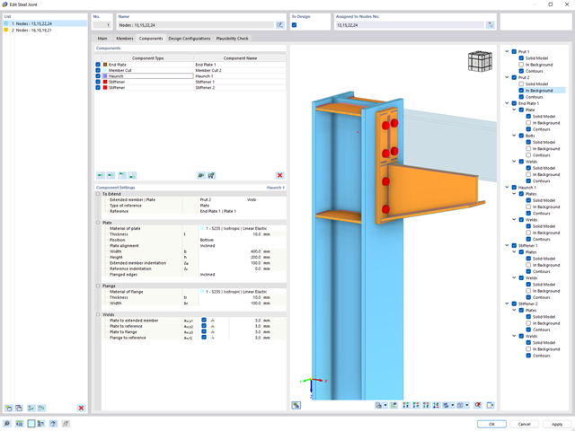
- Wybór węzłów w modelu RFEM, automatyczne rozpoznawanie i przydzielanie prętów połączonych z wybranym węzłem
- Dostępnych jest wiele wstępnie zdefiniowanych elementów ułatwiających wprowadzanie typowych komponentów połączeń (np. blachy czołowe, żebra usztywniające)
- Uniwersalne komponenty bazowe (płyty, spoiny, płaszczyzny pomocnicze) do odwzorowania złożonych geometrii połączeń
- Użytkownik nie musi ręcznie edytować modelu MES połączenia, podstawowe ustawienia obliczeń można zmienić w oknie konfiguracji połączenia
- Automatyczne dostosowywanie geometrii połączenia, nawet w przypadku późniejszej edycji prętów, z uwagi na parametryczną definicję położenia komponentów względem siebie
- Równolegle do wprowadzania danych program przeprowadza kontrolę poprawności, aby szybko wykryć brakujące dane wejściowe lub kolizje elementów.
- Wizualizacja geometrii połączenia, która jest aktualizowana równolegle z wprowadzaniem danych
Program wspiera Cię: Moduł określa siły w śrubach na podstawie modelu analitycznego ES i analizuje je automatycznie. Rozszerzenie przeprowadza obliczenia nośności śrub dla przypadków uszkodzeń, takich jak rozciąganie, ścinanie, docisk otworu i przebicie, zgodnie z normą i wyświetla w przejrzysty sposób wszystkie wymagane współczynniki.
Chcesz przeprowadzić wymiarowanie spoin? Spoiny są modelowane jako sprężysto-plastyczne elementy powierzchniowe, a ich naprężenia są odczytywane z modelu analitycznego ES. Kryterium plastyczności ma reprezentować zniszczenie zgodnie z AISC J2-4, J2-5 (wytrzymałość spoin) i J2-2 (wytrzymałość metalu podstawowego). Obliczenia można przeprowadzić z zastosowaniem częściowych współczynników bezpieczeństwa określonych w załączniku krajowym do normy EN 1993-1-8.
Płyty w połączeniu są wymiarowane w sposób plastyczny poprzez porównanie istniejącego odkształcenia plastycznego z dopuszczalnym odkształceniem plastycznym. Domyślne ustawienie wynosi 5% zgodnie z EN 1993-1-5, Załącznik C, ale można to zmienić według specyfikacji użytkownika, a także 5% dla AISC 360.
Wszystkie istotne wyniki można wyświetlić w modelu ES. W takim przypadku można filtrować wyniki osobno według odpowiednich komponentów.
Ponadto program RFEM zapewnia wszystkie kontrole obliczeń w formie tabelarycznej wraz z wyświetlaniem zastosowanych wzorów. W razie potrzeby tabele wyników można przenieść do protokołu wydruku programu RFEM.

- 002108
- Ogólne informacje
- Optymalizacja i koszty | Szacowanie emisji CO2 RFEM 6
- Optymalizacja i koszty | Szacowanie emisji CO2 RSTAB 9
- Technologia sztucznej inteligencji (AI): Optymalizacja roju cząstek (PSO)
- Optymalizacja konstrukcji ze względu na minimalny ciężar lub deformację
- Możliwość zastosowania dowolnej liczby parametrów optymalizacyjnych
- Określanie zakresów zmiennych
- Optymalizacja przekrojów i materiałów
- Typy definicji parametrów
- Optymalizacja | Rosnąco, czyli optymalizacja | Malejąca
- Zastosowanie parametrycznych modeli i bloków
- Parametryzacja bloków w języku JavaScript na podstawie kodu
- Optymalizacja z uwzględnieniem wyników obliczeń
- Tabelaryczne przedstawienie najlepszych mutacji modelu
- Wyświetlanie w czasie rzeczywistym mutacji modelu w procesie optymalizacji
- Kalkulacja kosztów modelu dzięki zadanym cenom jednostkowym
- Określanie potencjału tworzenia efektu cieplarnianego (GWP-global warming potential) na etapie tworzenia modelu poprzez szacowanie równoważnej emisji CO2
- Określanie jednostkowych wskaźników zależnych od masy, objętości i powierzchni (cena i emisja CO2)

- 002109
- Ogólne informacje
- Optymalizacja i koszty | Szacowanie emisji CO2 RFEM 6
- Optymalizacja i koszty | Szacowanie emisji CO2 RSTAB 9
Masz pytania dotyczące programu? Optymalizacja konstrukcji w programach RFEM i RSTAB jest uzupełnieniem parametrycznego wprowadzania danych. Jest to proces równoległy, niezależny od rzeczywistych obliczeń modelu wraz ze wszystkimi jego zwykłymi definicjami obliczeń i obliczeń. Rozszerzenie zakłada, że model lub blok jest zbudowany w kontekście parametrycznym i jest kontrolowany przez globalne parametry kontrolne typu "optymalizacja". Dlatego te parametry kontrolne mają dolną i górną granicę oraz wielkość kroku w celu ograniczenia zakresu optymalizacji. Aby znaleźć optymalne wartości parametrów kontrolnych, należy określić kryterium optymalizacji (na przykład minimalny ciężar) przy wyborze metody optymalizacji (na przykład optymalizacja roju cząstek).
Oszacowanie kosztów i emisji CO2 można znaleźć już w definicjach materiałów. Obie opcje można aktywować osobno w każdej definicji materiału. Oszacowanie oparte jest na koszcie jednostkowym lub jednostkowej wartości emisji dla prętów, powierzchni oraz brył. W tym przypadku można wybrać, czy jednostki mają zostać podane według masy, objętości czy powierzchni.

- 002110
- Ogólne informacje
- Optymalizacja i koszty | Szacowanie emisji CO2 RFEM 6
- Optymalizacja i koszty | Szacowanie emisji CO2 RSTAB 9
Istnieją dwie metody optymalizacji, dzięki którym można znaleźć optymalne wartości parametrów według kryterium ciężaru lub odkształcenia.
Najbardziej wydajną metodą o najkrótszym czasie obliczeń jest optymalizacja roju cząstek zbliżona do naturalnej (PSO). Czy słyszałeś lub czytałeś o tym? Ta technologia sztucznej inteligencji (AI) ma silną analogię do zachowania stad zwierząt szukających miejsca odpoczynku. W takich rojach można znaleźć wiele osób (por. rozwiązanie optymalizacyjne - na przykład waga), które lubią przebywać w grupie i podążać za ruchem grupy. Załóżmy, że każdy pręt roju musi zostać poddany spoczynkowi w optymalnym miejscu (por. najlepsze rozwiązanie - na przykład najniższa waga). Potrzeba ta wzrasta wraz ze zbliżaniem się do miejsca odpoczynku. Na zachowanie roju mają zatem wpływ również właściwości przestrzeni (por. wykres wyników).
Dlaczego wycieczka do biologii? Po prostu - proces PSO w RFEM lub RSTAB przebiega w podobny sposób. Proces obliczeń rozpoczyna się od wyniku optymalizacji poprzez losowe przypisanie parametrów, które mają zostać zoptymalizowane. Wielokrotnie określa nowe wyniki optymalizacji ze zróżnicowanymi wartościami parametrów, które opierają się na doświadczeniach z wcześniej przeprowadzonych mutacji modelu. Proces jest kontynuowany do momentu osiągnięcia określonej liczby możliwych mutacji modelu.
Jako alternatywa dla tej metody program oferuje również metodę przetwarzania wsadowego. Metoda ta ma na celu sprawdzenie wszystkich możliwych mutacji modelu poprzez losowe określanie wartości parametrów optymalizacji, aż do osiągnięcia określonej liczby możliwych mutacji modelu.
Po obliczeniu mutacji modelu obydwa warianty sprawdzają również odpowiednie aktywowane wyniki obliczeń rozszerzeń. Ponadto zapisuje on wariant z odpowiednim wynikiem optymalizacji i przypisaniem wartości parametrów optymalizacji, jeżeli wykorzystanie jest < 1.
Na podstawie odpowiednich sum poszczególnych materiałów można określić szacunkowe koszty całkowite i emisję. Na sumę materiałów składają się zależne od ciężaru, objętości i powierzchnie elementów prętowych, powierzchniowych i bryłowych.

- Definiowanie naprężeń na przykładzie sprężysto-plastycznego modelu materiałowego
- Wymiarowanie murowych konstrukcji tarczowych na ściskanie i ścinanie na modelu budynku lub na pojedynczym modelu
- Automatyczne określanie sztywności przegubu ściana-płyta
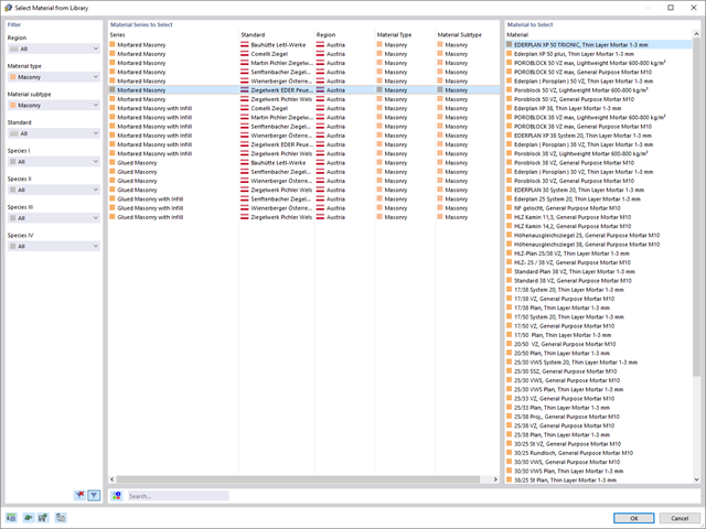
- Obszerna baza danych materiałów o prawie wszystkich kombinacjach kamienia i zapraw dostępnych na rynku austriackim (asortyment jest stale poszerzany, również dla innych krajów)
- Automatyczne określanie wartości materiałów zgodnie z Eurokodem 6 (ÖN EN 1996‑X)
- Możliwość przeprowadzenia analizy pushover
Konstrukcję wprowadza się i modeluje się bezpośrednio w programie RFEM. Model materiałowy muru można połączyć ze wszystkimi popularnymi rozszerzeniami dla programu RFEM. Umożliwia to projektowanie całych modeli budynków w połączeniu z murem.
Program automatycznie określa wszystkie parametry wymagane do obliczeń na podstawie wprowadzonych danych materiału. Następnie generowane są krzywe naprężenie-odkształcenie dla każdego elementu skończonego.
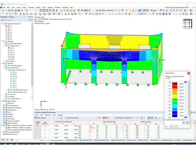
Czy projekt zakończył się sukcesem? Następnie po prostu usiądź i zrelaksuj się. Również tutaj można korzystać z licznych funkcji programu RFEM. Program podaje maksymalne naprężenia powierzchni murowanych, dzięki czemu można szczegółowo wyświetlić wyniki w każdym punkcie siatki ES.
Ponadto można wstawiać przekroje w celu przeprowadzenia szczegółowej analizy poszczególnych obszarów. Na podstawie przedstawionych obszarów uplastycznienia można oszacować zarysowania w murze.

- 002161
- Ogólne informacje
- Optymalizacja i koszty | Szacowanie emisji CO2 RFEM 6
- Optymalizacja i koszty | Szacowanie emisji CO2 RSTAB 9
Obie metody optymalizacji mają jedną wspólną cechę. Na końcu procesu wyświetlają listę wariacji modelu na podstawie przechowywanych danych. Można tu znaleźć szczegóły na temat wyniku decydującego dla optymalizacji i odpowiadające mu wartości parametrów. Lista jest zorganizowana w porządku malejącym. Zakładane najlepsze rozwiązanie znajduje się na górze. W takim przypadku wynik optymalizacji wraz z wyznaczoną wartością jest najbardziej zbliżony do kryterium optymalizacji. Wszystkie dodatkowe wyniki pokazują wykorzystanie < 1. Ponadto, po zakończeniu analizy, program dostosuje wartości na globalnej liście parametrów, aby odpowiadały tym dla optymalnego rozwiązania.
W oknach dialogowych materiałów znajdują się dodatkowe zakładki "Oszacowanie kosztów" i "Oszacowanie emisji CO2". Tutaj wyświetlane są indywidualne szacunkowe sumy przydzielonych prętów, powierzchni i objętości na jednostkę masy, objętości i powierzchni. Dodatkowo zakładki te podają całkowity koszt i emisję wszystkich przydzielonych do konstrukcji materiałów. Zapewnia to dobry przegląd projektu.
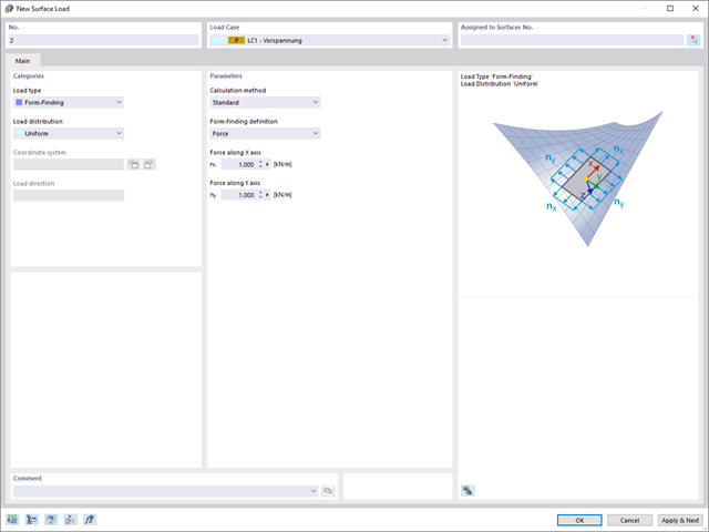
Po aktywowaniu rozszerzenia Form-Finding w Danych ogólnych, efekt znajdowania kształtu jest przypisywany do przypadków obciążeń z kategorią przypadków obciążenia "Sprężenie" w połączeniu z obciążeniami od znajdowania kształtu od pręta, powierzchni i bryły wczytaj katalog. Jest to przypadek obciążenia wstępnego naprężenia. Przekształca się on zatem w analizę znajdowania kształtu dla całego modelu ze zdefiniowanymi w nim wszystkimi elementami prętowymi, powierzchniowymi i bryłowymi. Do znajdowania kształtu odpowiednich elementów prętowych i membranowych dochodzi się w całym modelu za pomocą specjalnych obciążeń w zakresie znajdowania kształtu i regularnych definicji obciążeń. Te obciążenia znajdowania kształtu opisują oczekiwany stan odkształcenia lub siły po wyszukaniu kształtu w elementach. Obciążenia regularne opisują zewnętrzne obciążenie całego układu.