44 Wyniki
Wyświetl wyniki:
Sortuj według:

W rozszerzeniu Analiza geotechniczna dostępny jest wysokiej jakości model materiałowy "Zmodyfikowany model gruntu twardniejącego". Ten model materiałowy jest odpowiedni dla różnych gruntów i jest w stanie odpowiednio odwzorować następujące właściwości rzeczywistego gruntu.
- Zależność naprężenia od sztywności gruntu
- Zależność ścieżki obciążenia od sztywności gruntu
- Odkształcenia plastyczne jeszcze przed osiągnięciem warunku granicznego
- Wzrost wytrzymałości na ścinanie wraz ze wzrostem zagęszczenia siatki
- Wzrost granicy plastyczności wraz ze wzrostem naprężenia, aż do osiągnięcia granicznego warunku plastyczności
- Kryterium uszkodzenia według Mohra-Coulomba
Więcej informacji na temat tego modelu materiałowego oraz definicji danych wejściowych w programie RFEM można znaleźć w odpowiednim rozdziale instrukcji online rozszerzenia Analiza geotechniczna.
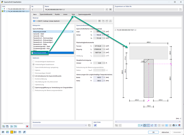
W rozszerzeniu Analiza etapów budowy (CSA) można używać przekrojów złożonych, dzięki zastosowaniu przekrojów etapowanych. Ten typ przekroju umożliwia aktywację lub dezaktywację poszczególnych części przekroju typu "Parametryczny - Masywny II" na poszczególnych etapach budowy.
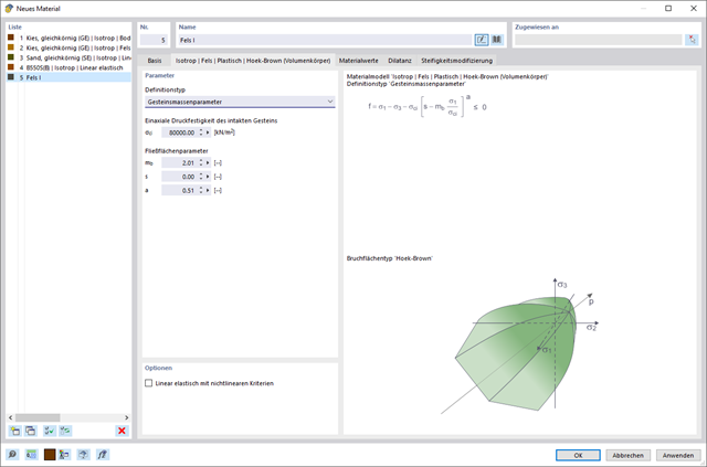
W rozszerzeniu Analiza geotechniczna dostępny jest model Hoek'a-Brown'a. Model wykazuje zachowanie materiału liniowo-sprężystego idealnie plastycznego. Jego nieliniowe kryterium wytrzymałości jest najczęściej stosowanym kryterium zniszczenia skał.
Parametry materiału można wprowadzić bezpośrednio za pomocą
- parametrów skały lub alternatywnie poprzez
- klasyfikację GSI.
opisane.
Weiterführende Informationen zu diesem Materialmodell und der Definition der Eingabe in RFEM finden Sie im entsprechenden Kapitel im Online-Handbuch für das Add-On Geotechnische Analyse: Model Hoeka-Browna .
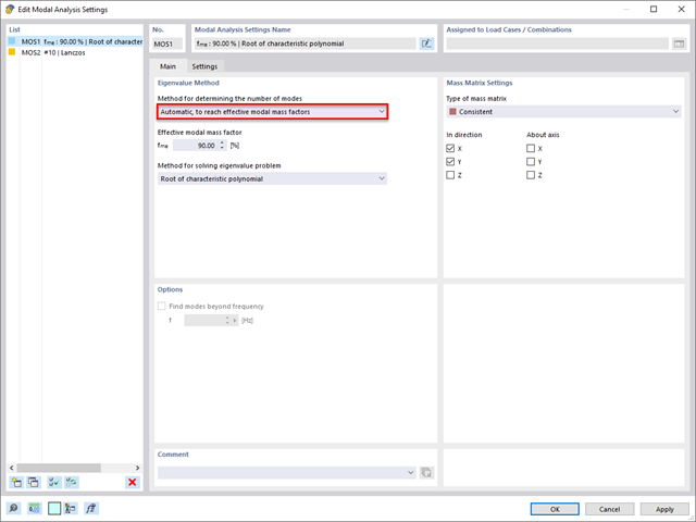
Rozszerzenie Analiza modalna umożliwia automatyczne zwiększanie poszukiwanych wartości własnych do momentu osiągnięcia zdefiniowanego współczynnika efektywnej masy modalnej. Uwzględniane są wszystkie kierunki translacyjne, które zostały aktywowane jako masy do analizy modalnej.
W ten sposób można łatwo obliczyć wymagane 90% efektywnej masy modalnej dla metody spektrum odpowiedzi.

W przypadku analizy spektrum odpowiedzi modeli budynków można wyświetlić współczynniki wrażliwości dla kierunków poziomych według kondygnacji.
Dzięki tym kluczowym wartościom można zinterpretować wrażliwość na efekty stateczności.
.png?mw=640&hash=403c565ab80c4dd45c2d1356634fb74a90428b70)
W bibliotece konstrukcji warstwowych dostępni są następujący producenci drewna klejonego krzyżowo:
- Binderholz (USA)
- KLH (USA, CAN)
- Kalesnikoff (USA, CAN)
- Nordic Structures (USA, CAN)
- Mercer Mass Timber
- SmartLam
- Sterling Structural
- Konstrukcje nośne wymienione w Lignatec wydanie 32 "Drewno klejone krzyżowo z produkcji szwajcarskiej"
Wczytanie konstrukcji z biblioteki konstrukcji warstw powoduje automatyczne przejęcie wszystkich istotnych parametrów. Biblioteka jest stale aktualizowana.
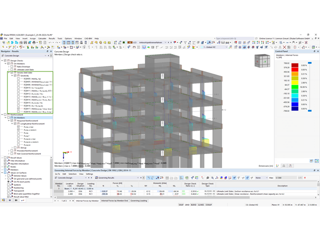
W rozszerzeniu Projektowanie konstrukcji betonowych można przeprowadzać obliczenia sejsmiczne dla prętów żelbetowych zgodnie z EC 8. Są to między innymi następujące funkcje:
- Konfiguracje obliczeń sejsmicznych
- Rozróżnianie klas ciągliwości DCL, DCM, DCH
- Możliwość przeniesienia współczynnika odpowiedzi z analizy dynamicznej
- Sprawdzenie wartości granicznej współczynnika odpowiedzi
- Weryfikacja nośności dla "Wytrzymały słup - słaba belka"
- Uszczegółowienie i reguły szczególne dla współczynnika ciągliwości krzywizny
- Uszczegółowienie i reguły szczególne dla ciągliwości lokalnej
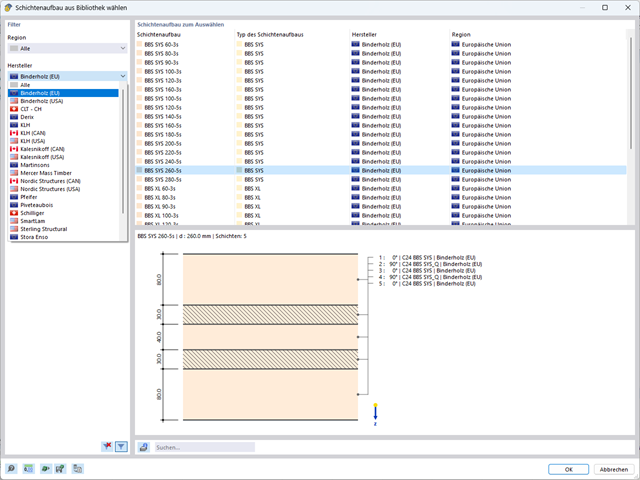
W programie RFEM zaimplementowano bibliotekę płyt z drewna klejonego krzyżowo, z której można importować konstrukcje warstwowe różnych producentów (np. Binderholz, KLH, Piveteaubois, Södra, Züblin Timber, Schilliger, Stora Enso). Oprócz grubości i materiałów warstw podane są również informacje o redukcji sztywności i łączeniu wąskich boków.
Przejdź do filmu.png?mw=640&hash=55038d2a1591f62179796666cb9b2fede0274e19)
Graficzne i tabelaryczne wyświetlanie wyników dla deformacji, naprężeń i odkształceń pomaga określić bryłę gruntu. Aby to osiągnąć, skorzystaj ze specjalnych kryteriów filtrowania, które umożliwiają wybór określonych wyników.
Program na pewno cię nie zawiedzie. Jeśli chcesz graficznie ocenić wyniki w bryłach gruntu, dostępne są obiekty pomocnicze. Na przykład można zdefiniować płaszczyzny przycinania. Umożliwia to przeglądanie odpowiednich wyników na dowolnej płaszczyźnie bryły gruntu.
I nie tylko to. Wykorzystanie przekrojów wyników i brył przycinania ułatwia graficzną analizę brył gruntu.
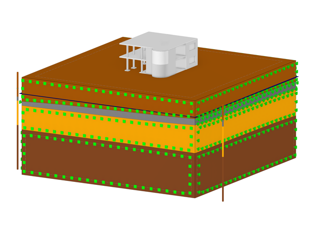
Wiesz już, że grunt i konstrukcję można modelować i analizować w całym modelu. Oznacza to, że wyraźnie uwzględniono interakcję gleba-konstrukcja. Dostosowanie jednego elementu konstrukcyjnego prowadzi do natychmiastowego prawidłowego uwzględnienia w analizie i wynikach dla całego układu gruntu i konstrukcji.
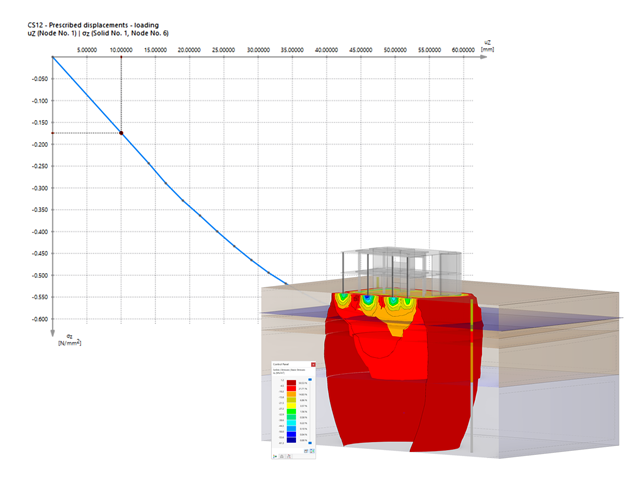
Czy jesteś gotowy na ocenę? Skorzystaj z wykresów obliczeniowych, które pokazują rozkład określonego wyniku podczas obliczeń.
Przypisanie osi pionowej i poziomej wykresu obliczeniowego można dowolnie definiować. Umożliwia to np. wyświetlenie przebiegu osiadania określonego węzła w zależności od obciążenia.
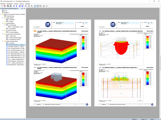
Twoje dane są zawsze dokumentowane w wielojęzycznym raporcie. W każdej chwili możesz dostosować treść i zapisać ją jako szablon. W raporcie można również za pomocą kilku kliknięć umieścić grafiki, teksty, wzory MathML i dokumenty PDF.
Wprowadzenie i modelowanie bryły gruntowej bezpośrednio w programie RFEM. Modele materiałów gruntowych można łączyć ze wszystkimi popularnymi rozszerzeniami dla programu RFEM.
Umożliwia to łatwą analizę całych modeli z pełną prezentacją interakcji grunt-konstrukcja.
Wszystkie parametry wymagane do obliczeń są określane automatycznie na podstawie wprowadzonych danych materiałowych. Następnie program generuje krzywe naprężenie-odkształcenie dla każdego elementu ES.
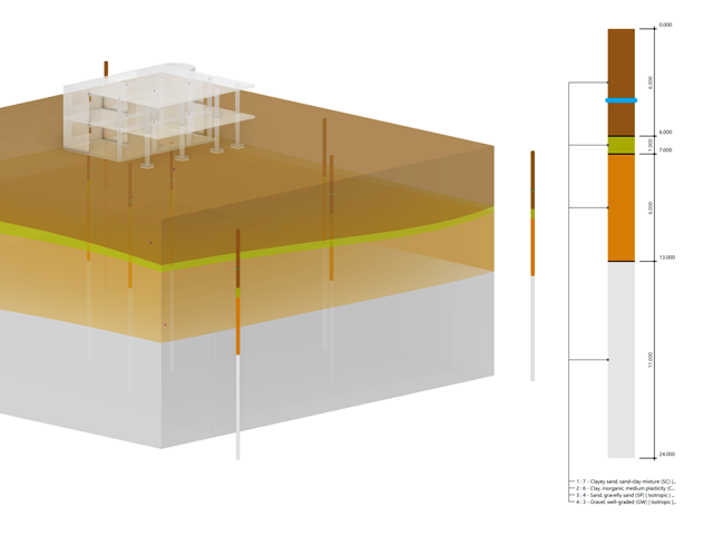
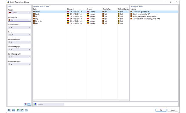
Czy wiecie, że...? Uwarstwienie gruntu, pobrane z raportów o podłożu gruntowym w miejscach wychodni, można wprowadzić bezpośrednio do programu w postaci próbek gruntu. Przypisz badane materiały gruntowe wraz z ich właściwościami do warstw.
Za pomocą danych tabelarycznych i okna dialogowego edycji można zdefiniować próbkę. Można również określić poziom wód gruntowych w próbkach gruntu.
Bryły gruntu, które mają zostać przeanalizowane, są sumowane w masywach gruntu.
Próbki gruntu należy wykorzystać jako podstawę do zdefiniowania masywu gruntowego. W ten sposób program umożliwia generowanie masywu w sposób przyjazny dla użytkownika, w tym automatyczne określanie granic faz na podstawie danych z próbki, a także poziomu wód gruntowych i podpór powierzchni granicznej.
Masywy gruntowe umożliwiają określenie docelowego rozmiaru siatki ES niezależnie od ustawień globalnych dla reszty konstrukcji. Dzięki temu w całym modelu można uwzględnić różne wymagania dotyczące budynku i gruntu.
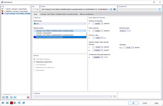
Czy chcesz modelować i analizować zachowanie bryły gruntowej? Aby to zapewnić, w programie RFEM zaimplementowano odpowiednie modele materiałowe.
Można użyć zmodyfikowanego modelu Mohra-Coulomba z liniowo-sprężystym modelem idealnie plastycznym lub nieliniowo sprężystym modelem z edometryczną relacją naprężenie-odkształcenie. Kryterium graniczne, które opisuje przejście od obszaru sprężystości do obszaru płynięcia plastycznego, jest zdefiniowane według Mohra-Coulomba.
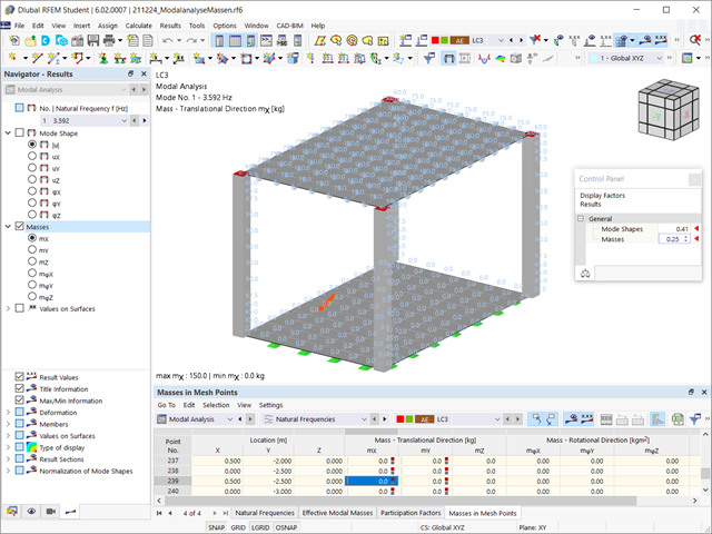
Czy odkryłeś już tabelaryczne i graficzne przedstawianie mas w punktach siatki? Po prawej, jest to również jeden z wyników analizy modalnej w programie RFEM 6. W ten sposób można sprawdzić importowane masy, które zależą od różnych ustawień analizy modalnej. Mogą być one wyświetlane w zakładce Masy w punktach siatki tabeli Wyniki. Tabela zawiera przegląd następujących wyników: Masa - kierunek przesuwny (mX, mY, mZ ), Masa - kierunek obrotowy (mφX, mφY, mφZ ) oraz suma mas. Czy nie byłoby lepiej, gdybyś jak najszybciej przeprowadził ocenę graficzną? Następnie można również wyświetlić graficznie masy w punktach siatki.
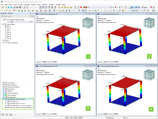
Jak już wiesz, po pomyślnym zakończeniu obliczeń wyniki przypadku obciążenia w Analizie modalnej są wyświetlane w programie. Die erste Eigenform ist für Sie also sofort grafisch oder animiert zu sehen. Dabei können Sie die Darstellung der Eigenformnormierung komfortabel anpassen. Erledigen Sie das am besten direkt im Ergebnisnavigator, wo Sie zur Visualisierung der Eigenformen eine von vier Optionen auswählen:
- Wert des Eigenformvektors uj auf 1 skalieren (berücksichtigt nur die Translationskomponenten)
- Auswahl der maximalen Translationskomponente des Eigenvektors und Einstellung auf 1
- Betrachtung der gesamten Eigenform (inklusive der Rotationskomponenten), Auswahl des Maximums und Einstellung auf 1
- Setzen der modalen Massen mi für jeden Eigenwert auf 1 kg
Ausführlichere Erläuterungen der Normierung der Eigenformen finden Sie hier: Instrukcja online .
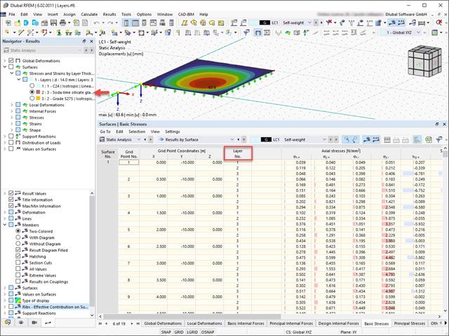
Wyniki naprężeń i odkształceń według powierzchni można wyświetlić w tabeli wyników powierzchni zgodnie z grubością warstwy.
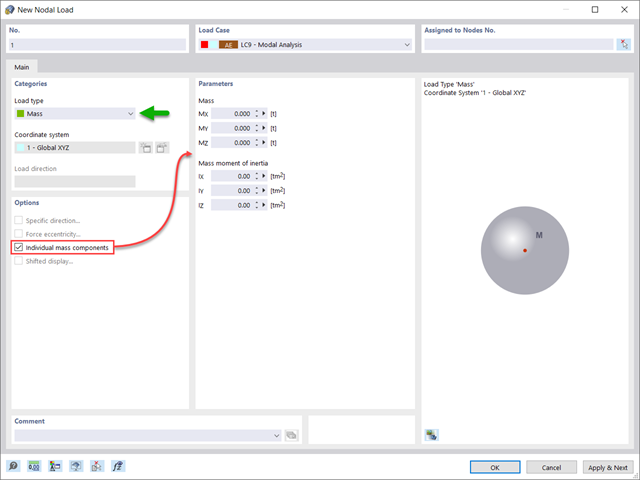
Czy oprócz obciążeń statycznych chcesz uwzględnić również inne obciążenia jako masy? Program umożliwia to dla obciążeń węzłowych, prętowych, liniowych i powierzchniowych. W tym celu podczas definiowania obciążenia należy wybrać typ Obciążenie masą. Dla takich obciążeń należy zdefiniować masę lub składowe masy w kierunkach X, Y i Z. W przypadku mas węzłowych można dodatkowo zdefiniować momenty bezwładności X, Y i Z w celu modelowania bardziej złożonych punktów mas.
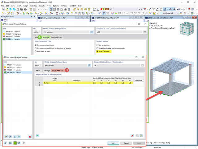
Często zachodzi potrzeba pominięcia mas. Dzieje się tak zwłaszcza w przypadku, gdy wyniki analizy modalnej mają być wykorzystane do analizy sejsmicznej. W tym celu wymagane jest 90% efektywnej masy modalnej w każdym kierunku. Pozwala to na pominięcie masy we wszystkich utwierdzonych podporach węzłowych i liniowych. Program automatycznie dezaktywuje powiązane masy.
Obiekty, których masy mają zostać pominięte w analizie modalnej, można również wybrać ręcznie. Dla lepszego widoku pokazaliśmy to ostatnie na rysunku. W wyniku wyboru przez użytkownika obiektów masowych wraz z skojarzonymi z nimi składowymi masowymi można pominąć masy.
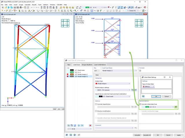
Podczas definiowania danych wejściowych dla przypadku obciążenia analizy modalnej można uwzględnić przypadek obciążenia, którego sztywności reprezentują początkową pozycję analizy modalnej. Jak to zrobić? Jak pokazano na rysunku, należy wybrać opcję "Uwzględnij stan początkowy z". Teraz otwórz okno dialogowe "Ustawienia stanu początkowego" i zdefiniuj typ Sztywność jako stan początkowy. W tym przypadku obciążenia, który jest stanem początkowym branym pod uwagę, można uwzględnić sztywność układu konstrukcyjnego, gdy pręty rozciągane ulegają uszkodzeniu. Celem tego wszystkiego: Sztywność z tego przypadku obciążenia jest uwzględniana w analizie modalnej. W ten sposób uzyskuje się wyraźnie elastyczny system.
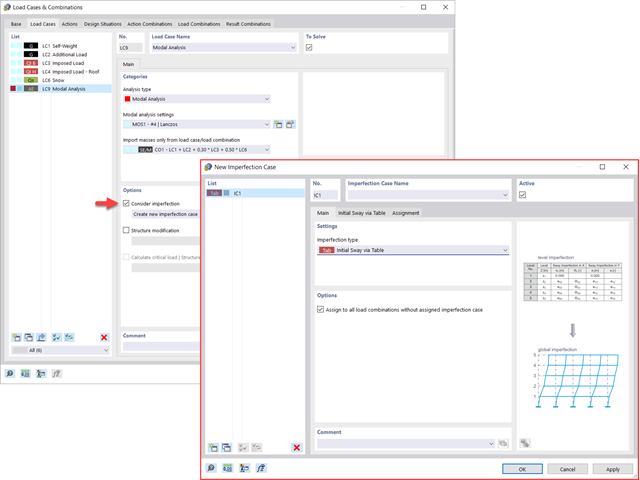
Widać to już na obrazku: Imperfekcje można również uwzględnić podczas definiowania przypadku obciążenia w analizie modalnej. Typy imperfekcji, które mogą być stosowane w analizie modalnej, to obciążenia hipotetyczne z przypadku obciążenia, początkowe przemieszczenie w tabeli, odkształcenie statyczne, postać wyboczeniowa, postać dynamiczna oraz grupa przypadków imperfekcji.
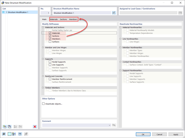
Czy wiecie, że...? W przypadkach obciążeń typu Analiza modalna można z łatwością wprowadzać zmiany konstrukcyjne. Pozwala to na przykład na indywidualne dostosowanie sztywności materiałów, przekrojów, prętów, powierzchni, przegubów i podpór. W przypadku niektórych rozszerzeń można również modyfikować sztywności. Po wybraniu obiektów ich właściwości sztywności są dostosowywane do typu obiektu. W ten sposób można je zdefiniować w osobnych zakładkach.
Czy chcesz przeanalizować uszkodzenie obiektu (na przykład słupa) w analizie modalnej? Jest to również możliwe bez żadnych problemów. Wystarczy przejść do okna Modyfikacja konstrukcji i dezaktywować odpowiednie obiekty.
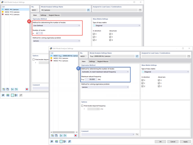
Twoim celem jest określenie liczby postaci drgań własnych? Program oferuje dwie metody. Z jednej strony, można ręcznie zdefiniować liczbę najmniejszych kształtów drgań, które mają zostać obliczone. W tym przypadku liczba dostępnych kształtów postaci zależy od stopni swobody (tzn. liczby punktów mas swobodnych pomnożonych przez liczbę kierunków, w których działają masy). Jest to jednak ograniczone do 9999. Z drugiej strony, maksymalną częstotliwość drgań własnych można ustawić w taki sposób, w jaki program określił kształty automatycznie, aż do osiągnięcia zadanej częstotliwości drgań własnych.
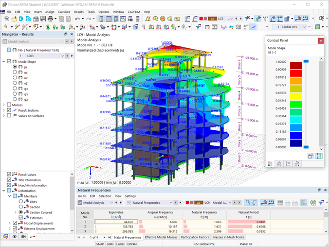
Czy obliczenia się zakończyły? Wyniki analizy modalnej są wówczas dostępne zarówno w formie graficznej, jak i tabelarycznej. Wyświetl tabele wyników dla przypadku obciążenia lub przypadków obciążeń analizy modalnej. Dzięki temu na pierwszy rzut oka można zobaczyć wartości własne, częstotliwości kątowe, częstotliwości i okresy drgań własnych konstrukcji. W przejrzysty sposób wyświetlane są również efektywne masy modalne, modalne współczynniki masy i współczynniki udziału.
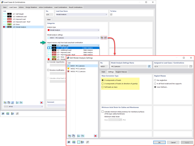
Dostępnych jest kilka opcji definiowania mas dla analizy modalnej. Masy od ciężaru własnego są uwzględniane automatycznie, natomiast obciążenia i masy można uwzględnić bezpośrednio w przypadku obciążenia typu analiza modalna. Potrzebujesz więcej opcji? Należy wybrać, czy obciążenia pełne mają być uwzględniane jako masy, składowe obciążenia w globalnym kierunku Z, czy tylko składowe obciążenia w kierunku siły ciężkości.
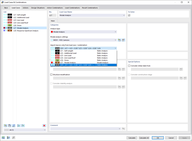
Program oferuje dodatkową lub alternatywną opcję importu mas: Ręczna definicja kombinacji obciążeń, począwszy od których masy są uwzględniane w analizie modalnej. Wybrałeś normę obliczeniową? Następnie można utworzyć sytuację obliczeniową typu Kombinacja mas sejsmicznych. W ten sposób program automatycznie oblicza sytuację masową dla analizy modalnej zgodnie z preferowaną normą obliczeniową. Innymi słowy: Program tworzy kombinację obciążeń na podstawie współczynników kombinacji wstępnie ustawionych dla wybranej normy. Zawiera on masy użyte do analizy modalnej.
W porównaniu z modułem dodatkowym RF-/DYNAM Pro-Natural Vibrations (RFEM 5/RSTAB 8) do rozszerzenia Analiza modalna dla programu RFEM 6/RSTAB 9 dodano następujące nowe funkcje:
- Predefiniowane współczynniki kombinacji dla różnych norm (EC 8, ASCE itp.)
- Opcjonalne pominięcie mas (na przykład masy fundamentów)
- Metody określania liczby postaci drgań własnych (liczba zdefiniowana przez użytkownika, liczba określana automatycznie - w celu osiągnięcia zadanych efektywnych współczynników masy modalnej, liczba określana automatycznie - w celu osiągnięcia maksymalnej częstotliwości drgań własnych)
- Wyniki w postaci mas modalnych, efektywnych mas modalnych, współczynników masy modalnej i współczynników udziału masy
- Tabelaryczne i graficzne przedstawienie mas w punktach siatki MES
- Różne opcje skalowania postaci drgań własnych w nawigatorze wyników
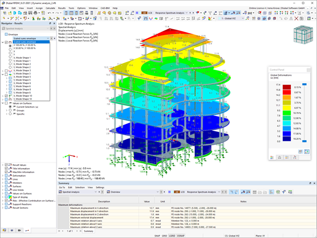
W porównaniu z modułem dodatkowym RF-/DYNAM Pro-Equivalent Loads (RFEM 5/RSTAB 8) do rozszerzenia Analiza spektrum odpowiedzi dla programu RFEM 6/RSTAB 9 dodano następujące nowe funkcje:
- Spektrum odpowiedzi z wielu norm (EN 1998, DIN 4149, IBC 2018 itd.)
- Spektrum odpowiedzi zdefiniowane przez użytkownika lub wygenerowane z akcelerogramów
- Możliwość zadania kierunkowego spektrum odpowiedzi
- Aby zapewnić przejrzystość wyniki są przechowywane łącznie, w jednym przypadku obciążenia, w ramach którego dostępne są różne poziomy wyświetlania
- Wpływ przypadkowych oddziaływań skręcających może być uwzględniany automatycznie
- Automatyczne kombinacje obciążeń sejsmicznych z innymi przypadkami obciążeń, możliwe do wykorzystania w wyjątkowej sytuacji obliczeniowej

W porównaniu z modułem dodatkowym RF-SOILIN (RFEM 5) do rozszerzenia Analiza geotechniczna dla programu RFEM 6 dodano następujące nowe funkcje:
- Tworzenie warstwowego gruntu jako modelu 3D z całości zdefiniowanych próbek gruntu
- Symulacja gruntu zgodnie z teorią Mohra-Coulomba
- Graficzne i tabelaryczne przedstawienie naprężeń i odkształceń na dowolnej głębokości gruntu
- Optymalne uwzględnienie interakcji gruntu i konstrukcji na podstawie modelu ogólnego