


The sensitivity coefficient θ is defined as follows [1]:
|
θ |
Interstory drift sensitivity coefficient |
|
Ptot |
Total gravity load at and above the story considered in the seismic design situation |
|
dr |
Design interstory drift, evaluated as the difference of the average lateral displacements ds at the top and bottom of the story under consideration; for this, the displacement is determined by using the linear design response spectrum with q = 1.0 |
|
Vtot |
Total seismic story shear determined by using the linear design response spectrum |
|
h |
Story height |
The second-order effects may be taken into account approximately by a factor equal to 1 / (1 − θ), if 0.1 < θ ≤ 0.2. For θ > 0.2, it is necessary to consider the geometric stiffness matrix when calculating eigenvalues and multi-modal response spectrum analysis.
Geometric Stiffness Matrix
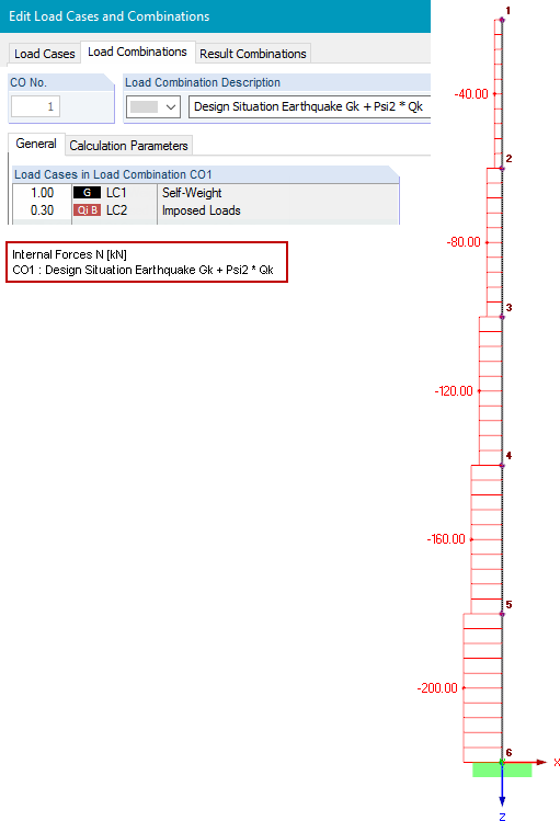
For dynamic analyses, the iterative calculations for the nonlinear determination of second-order theory are not suitable. The problem can be linearized, and it is sufficient to use the geometric stiffness matrix based on axial loads to consider the second-order theory. For this, it is assumed that the vertical loads do not change due to horizontal effects, and the deformations are small compared to the building dimensions [2]. The loads to be considered should correspond to those for the seismic design situations in accordance with EN 1990, Section 6.4.3.4 [3]:
|
Ed |
Design value of actions |
|
Gk,j |
Characteristic value of permanent action j |
|
Qk,i |
Characteristic value of variable action i |
|
Ψ2,i |
Factor for quasi-permanent values of variable actions i |
where
Ed = the design value of effects
Gk,j = the characteristic value of the permanent action j
Qk,i = the characteristic value of the variable action i
Ψ2,i = the factor for the quasi‑permanent values of variable actions i
Axial tensile forces increase the stiffness, for example, in a prestressed cable. Compression forces reduce the stiffness and can lead to a singularity in the stiffness matrix. The geometric stiffness Kg is not dependent on the mechanical properties of the structure, but only on the member length L and axial force N. To illustrate the basic problem, a simple example of a cantilever is displayed in Image 01. The individual mass points of the cantilever represent the individual stories of a building. The building is subjected to a dynamic analysis considering the second-order theory. The axial forces Ni on the individual stories i = 1…n result from the vertical forces in the seismic design situation (see Expression 2). The story height is defined by hi.
![Reduction of Building to Cantilever Structure: The individual mass points represent the floors. The deflection due to the normal compression forces shown in (a) is (b) converted into equivalent moments of displacement or shear forces [2].](/en/webimage/009762/2420261/01-en-png-12-png.png?mw=760&hash=1a55701832b7f5294a58c425fced514b7458a61b)
The geometric stiffness matrix Kg can be derived from the static equilibrium conditions:
For the purpose of simplification, only the degrees of freedom of the horizontal displacement are displayed here. The derivation shown is based on the overturning moment approach due to the linear displacement application. This is a simplification for the bending element, and an accurate assumption for the truss element. More precise determination of the geometric stiffness matrix for bending beams can be obtained using the cubic displacement approach or the analytical solution of the differential equation of the bending line. More detailed information and derivations are provided by Werkle [4]. The geometric stiffness matrix Kg is added to the system stiffness matrix K, and thus the modified stiffness matrix Kmod is obtained:
Kmod = K + Kg (4)
In the case of compression normal forces, this consequently leads to stiffness reduction.
Example: Natural Frequencies and Multi-Modal Response Spectrum Considering Second-Order Analysis
The following shows how the geometric stiffness matrix can be considered in RFEM and the RF-DYNAM Pro add-on modules. The cantilever shown in Image 01 is used as an example. The cantilever consists of five concentrated mass points. Here, 4,000 kg act in the global X-direction in each case.
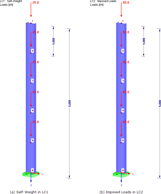
The cross‑section is IPE 300 made of S 235 material with Iy = 8,356 ∙ 10-5 m4 and E = 2.1 ∙ 1011 N/m². To be able to consider the geometric stiffness matrix in the dynamic analysis, a load combination is initially defined for the seismic design situation in the RFEM main program (see Equation 2).
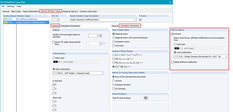
The RF‑DYNAM Pro – Natural Vibrations add‑on module allows you to determine natural frequencies, mode shapes, and effective modal masses of a structure, taking into account various stiffness modifications (see RF‑DYNAM Pro Manual [5], Chapter 2.4.7, and Technical Article [6]). Two natural vibration cases are defined. In NVC2, LC1 is imported in order to consider the geometric stiffness matrix and thus the second-order theory. For comparison, the NVC1 is defined, which does not include any stiffness modifications.
The following table includes the determined natural frequencies f [Hz], natural periods T [sec], and the acceleration values Sa [m/s²] based on the response spectrum, with and without the geometric stiffness matrix Kg resulting from the axial forces of CO1.
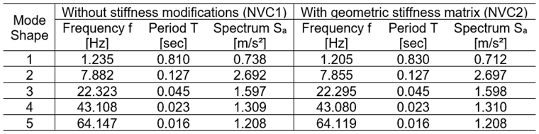
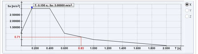
The multi-modal response spectrum analysis uses natural frequencies to determine the acceleration values from the defined response spectrum. The equivalent loads and the response spectrum internal forces are determined on the basis of these acceleration values. The graphic display of a user‑defined response spectrum is shown in Figure 06, and the acceleration values Sa [m/s²] determined from the response spectrum for each eigenvalue are listed in the table above.
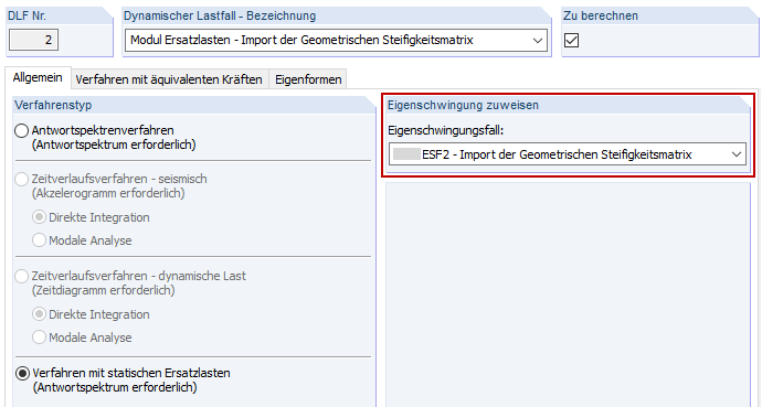
In order to ensure the correct allocation of the modified frequencies, the right natural vibration case (NVC) must be assigned to the dynamic load case (DLC).
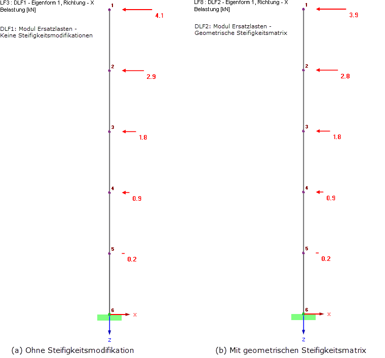
In the case of compression axial forces, the consideration of the geometric stiffness matrix leads to the reduction of the natural frequency, and can cause lower acceleration values Sa, as in our example. The modification of the natural frequencies alone is not enough to take the second-order theory into account; on the contrary, this may even lead to smaller results and thus be less reliable. It is very important also to use the modified stiffness matrix for the determination of internal forces and deformations. In RF-DYNAM Pro - Forced Vibrations, the modified stiffness is used automatically to determine the response spectrum results, because the calculation is performed within RF-DYNAM Pro. In RF-DYNAM Pro - Equivalent Loads, the equivalent loads are determined and exported as load cases into the main program RFEM. Therefore, the calculation is partially performed in RF-DYNAM Pro and partially in RFEM. The theoretical background for the equivalent load calculation is explained in the Manual RF-DYNAM Pro [5]. The verification example [7] shows the calculation on a specific example. The determined equivalent loads, with and without the geometric stiffness matrix, are displayed in Image 08.
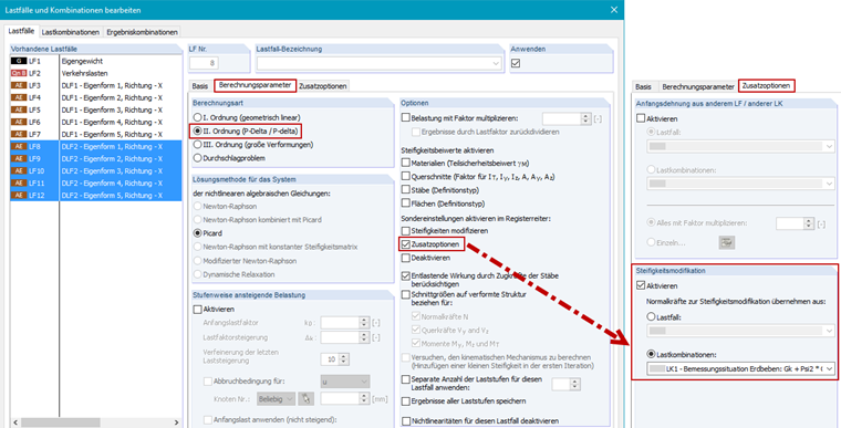
The export of the equivalent loads has many advantages, but the most important is the correct transfer of stiffness modifications in the load cases. The calculation parameters of the exported load cases must be adjusted as shown in Image 09.
The individual load cases are superimposed using the SRSS or CQC method. This is automatically set in RF-DYNAM Pro and exported into result combinations. The results with and without the geometric stiffness matrix are displayed in Image 10.
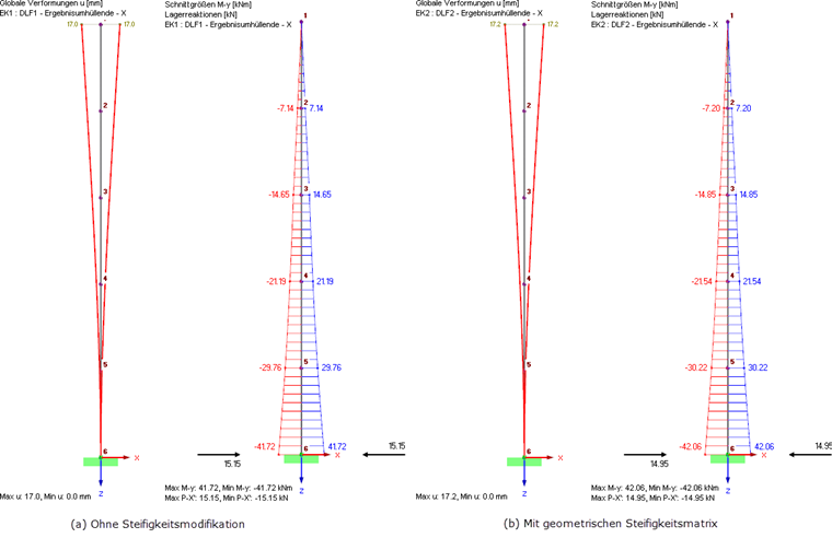
The consideration of the geometric stiffness matrix leads to larger deformations and internal forces. However, the effective equivalent loads and resulting support loads are slightly smaller when considering the geometric stiffness matrix.