The way to provide data obtained from field tests in the add-on and use the properties from soil samples to determine the soil massifs of interest was discussed in the Knowledge Base article "Creating Soil Body from Soil Samples in RFEM 6".
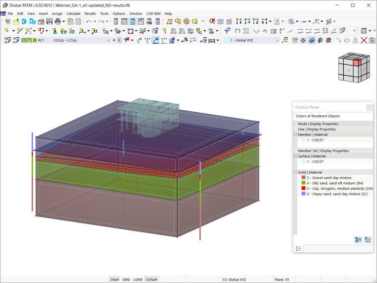
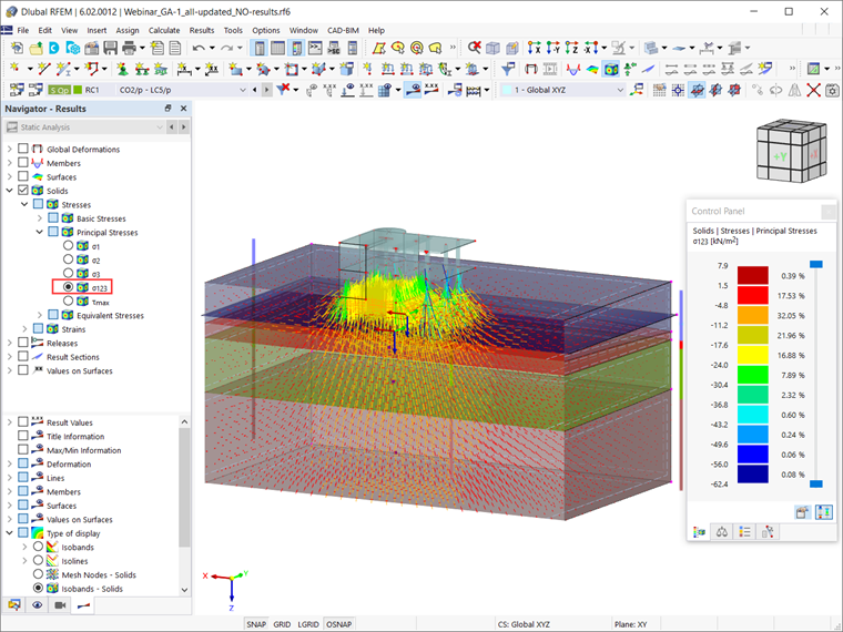
In a similar manner, Knowledge Base article "Geotechnical Analysis in RFEM 6" shows you how to create load cases, load combinations, and result combinations, and how to define analysis settings and parameters. Hence, assuming that the superstructure has been modeled, the soil massif of interest has been determined (Image 1), and the calculation has been initiated, this text will discuss the results of the analysis and their graphical and tabular display in the RFEM 6 program.
Stresses
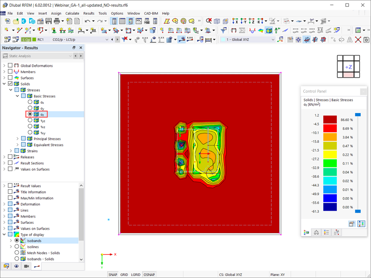
The first results to be considered in this article are the basic stresses in terms of the initial state; that is, the self-weight of the soil. As a result, the “Self-weight Soil” load case is selected in the drop-down menu of the toolbar, and the basic stresses σz are selected in the Results navigator.
This way, the graphical display of the basic stresses σz resulting from the self-weight of the soil is available in the workspace of the program, as shown in Image 2. These results are also available to you in tabular form in the Static Analysis table.
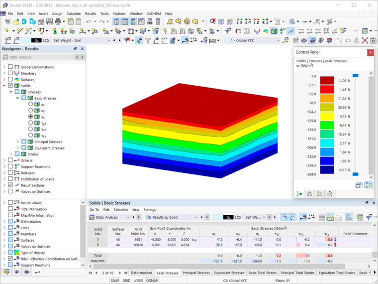
If you are interested in controlling the boundary surfaces, or, in other words, checking the dimensions of the soil massif, you can compare the basic stresses for the initial state with those for the leading load combination.
For that purpose, you should select LC 1 in the drop-down menu and check the stresses in the bottom soil surface. In this example, the difference between the results for the leading load combination (Image 3) and the initial state (Image 2) is no more than 10%. Hence, we can conclude that the dimensions of the soil massif are sufficient.
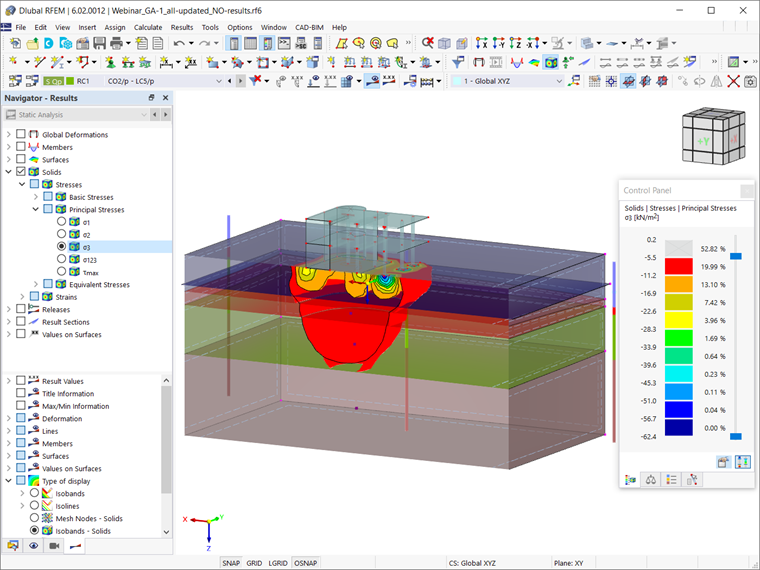
Next, you can check the principal stresses σ3 for the result combination in which the results from the initial state have been excluded. Thus, the stresses obtained are solely those from the leading load combination, or to be more specific, the stresses due to the construction of the building itself. To see the stresses in the soil solid in greater detail, you can create a clipping plane as shown in Image 4. As the image shows, the stresses in the soil are sufficiently far from the boundary surface.
You also can display the stresses’ trajectories in the soil solid, as shown in Image 5.
Another important result of the analysis is the contact stresses; that is, the stresses on the contact between the slab and the surfaces of the columns’ foundation on one hand, and the soil on the other. To display them in the correct manner, select “Isobands” as the display type. If you set the view in the model in the Z direction, you can see the contact stress as shown in Image 6.
Displacements
The results of the analysis include the displacements of the structure due to the applied loads. They can be displayed in both tabular and graphical form. For the latter, you must select the uz global deformations in the Results navigator. In the same way as discussed before, you can create a clipping plane and have a better view into the deformations. In Image 7, a clipping plane has been defined as a cut through the columns, which provides you with a three-dimensional view of the structure’s displacements into the soil. Thus, you can see that the foundation slab has a settlement curve that also affects the foundations of the columns, as well as the fact that neighboring foundations influence each other’s settlements.