88 Results
View Results:
Sort by:
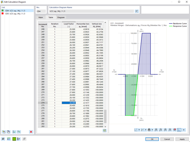
For calculation diagrams, you can use the "2D | Hinge" diagram type. These hinge diagrams show the hinge response of load situations for nonlinear hinges.
For calculations with several load situations, such as the case with the pushover analysis and time history analysis, you can evaluate the hinge condition in each load step.
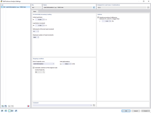
The pushover analysis is managed by a newly introduced analysis type in the load combinations. Here, you have access to the selection of the horizontal load distribution and direction, the selection of a constant load, the selection of the desired response spectrum for the determination of the target displacement, and the pushover analysis settings tailored to the pushover analysis.
In the pushover analysis settings, you can modify the increment of the increasing horizontal load and specify the stopping condition for the analysis. Furthermore, it is possible to easily adjust the precision for the iterative determination of the target displacement.
During the calculation, the selected horizontal load is increased in load steps. A static nonlinear analysis is carried out for each load step until reaching the specified limit condition.
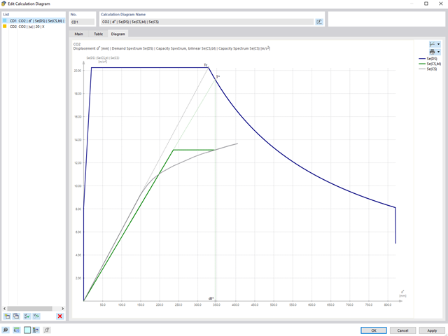
The results of the pushover analysis are extensive. On one hand, the structure is analyzed for its deformation behavior. This can be represented by a force-deformation line of the system (a capacity curve). On the other hand, the response spectrum effect can be displayed in the ADRS display (Acceleration-Displacement Response Spectrum). The target displacement is automatically determined in the program based on these two results. The process can be evaluated graphically and in tables.
The individual acceptance criteria can then be graphically evaluated and assessed (for the next load step of the target displacement, but also for all other load steps). The results of the static analysis are also available for the individual load steps.
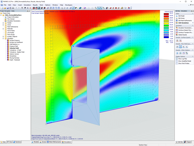
Use RWIND 2 Pro to easily apply a permeability to a surface. All you need is the definition of
- the Darcy coefficient D,
- the inertial coefficient I, and
- the length of the porous medium in the direction of flow L,
to define a pressure boundary condition between the front and back of a porous zone. Due to this setting, you obtain the flow through this zone with a two-part result display on both sides of the zone area.
But that's not all. Furthermore, the generation of a simplified model recognizes permeable zones and takes into account the corresponding openings in the model coating. Can you waive an elaborate geometric modeling of the porous element? Understandable – we have good news for you then! With a pure definition of the permeability parameters, you can avoid complex geometric modeling of the porous element. Use this feature to simulate permeable scaffolding, dust curtains, mesh structures, and so on.
More Information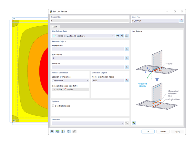
You probably already know that node, line, and surface releases are used to define transfer conditions between objects. For example, you can release members, surfaces, and solids from a line. It is also easily possible for the releases to have nonlinear properties, such as "Fixed if positive n", "Fixed if negative n", and so on.
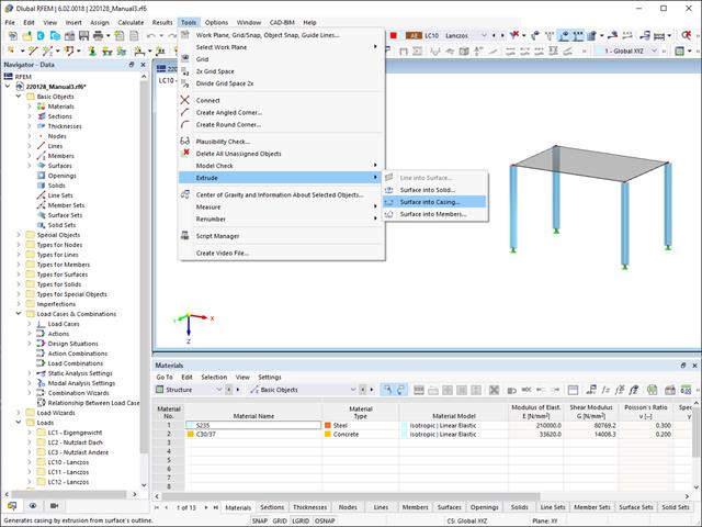
Extruding surfaces into a casing is also possible without any problems. Place the desired surface properties between the boundary lines of the surface and the copied lines. The program does the rest for you.

The soil solids that you want to analyze are summarized in soil massifs.
Use the soil samples as a basis for a definition of the respective soil massif. This way, the program allows for user-friendly generation of the massif, including the automatic determination of the layer interfaces from the sample data, as well as the groundwater level and the boundary surface supports.
Soil massifs provide you with the option to specify a target FE mesh size independently of the global setting for the rest of the structure. You can thus consider the various requirements of the building and soil in the entire model.
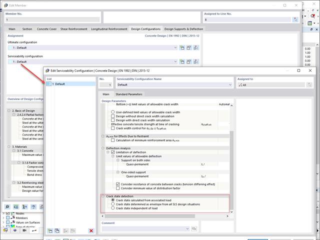
Various design parameters of the cross-sections can be adjusted in the serviceability limit state configuration. The applied cross-section condition for the deformation and crack width analysis can be controlled there.
For this, the following settings can be activated:
- Crack state calculated from associated load
- Crack state determined as an envelope from all SLS design situations
- Cracked state of cross-section - independent of load
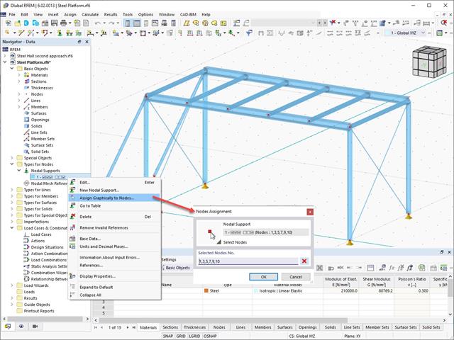
The object types listed below can be graphically assigned to the elements of the structure modeled in the program.
- Nodal supports
- Member shear panels
- Local reductions of member cross-sections
- Member transverse stiffeners
- Member longitudinal welds
- Effective lengths
- Boundary conditions
- Line supports
- Loads
- Member support
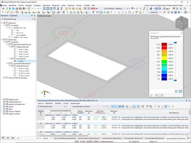
- Punching reinforcements
- Mesh refinements
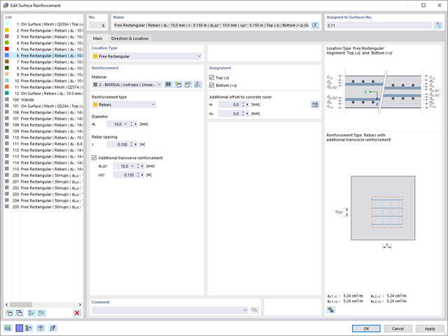
- Surface reinforcements
- Surface results adjustments
- Surface support
- Service classes
- Imperfections
.png?mw=640&hash=342149908caead326e60e26a2b5d05f7f46825cb)
Are you familiar with the Tsai-Wu material model? It combines plastic and orthotropic properties, which allows for special modeling of materials with anisotropic characteristics, such as fiber-reinforced plastics or timber.
If the material is plastified, the stresses remain constant. The redistribution is carried out according to the stiffnesses available in the individual directions. The elastic area corresponds to the Orthotropic | Linear Elastic (Solids) material model. For the plastic area, the yielding according to Tsai-Wu applies:
All strengths are defined positively. You can imagine the stress criterion as an elliptical surface within a six-dimensional space of stresses. If one of the three stress components is applied as a constant value, the surface can be projected onto a three-dimensional stress space.
If the value for fy(σ), according to the Tsai-Wu equation, plane stress condition, is smaller than 1, the stresses are in the elastic zone. The plastic area is reached as soon as fy (σ) = 1; values greater than 1 are not allowed. The model behavior is ideal-plastic, which means there is no stiffening.
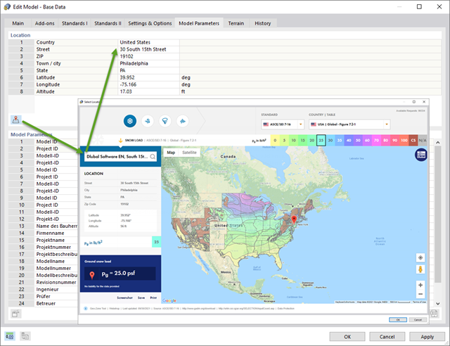
Always keep an eye on the natural conditions of your construction site by defining it on a digital map. The address data (including the altitude) as well as the snow load zone, wind zone, and seismic zone are imported automatically. The load wizard also uses this data.
The map is also displayed with the construction site marked in the "Model Parameters" tab.
Go to Explanatory Video
Compared to the RF-FORM-FINDING add-on module (RFEM 5), the following new features have been added to the Form-Finding add-on for RFEM 6:
- Specification of all form-finding load boundary conditions in one load case
- Storage of form-finding results as initial state for further model analysis
- Automatic assignment of the form-finding initial state via combination wizards to all load situations of a design situation
- Additional form-finding geometry boundary conditions for members (unstressed length, maximum vertical sag, low-point vertical sag)
- Additional form-finding load boundary conditions for members (maximum force in member, minimum force in member, horizontal tension component, tension at i-end, tension at j-end, minimum tension at i-end, minimum tension at j-end)
- Material types "Fabric" and "Foil" in material library
- Parallel form-findings in one model
- Simulation of sequentially building form-finding states in connection with the Construction Stages Analysis (CSA) add-on

Compared to the RF-/STEEL Warping Torsion add-on module (RFEM 5 / RSTAB 8), the following new features have been added to the Torsional Warping (7 DOF) add-on for RFEM 6 / RSTAB 9:
- Complete integration into the environment of RFEM 6 and RSTAB 9
- 7th degree of freedom is directly taken into account in the calculation of members in RFEM/RSTAB on the entire system
- No more need to define support conditions or spring stiffnesses for calculation on the simplified equivalent system
- Combination with other add-ons is possible, for example for the calculation of critical loads for torsional buckling and lateral-torsional buckling with stability analysis
- No restriction to thin-walled steel sections (it is also possible to calculate ideal overturning moments for beams with massive timber sections, for example)
Do you know exactly how the form-finding is performed? First, the form-finding process of the load cases with the load case category "Prestress" shifts the initial mesh geometry to an optimally balanced position by means of iterative calculation loops. For this task, the program uses the Updated Reference Strategy (URS) method by Prof. Bletzinger and Prof. Ramm. This technology is characterized by equilibrium shapes that, after the calculation, comply almost exactly with the initially specified form-finding boundary conditions (sag, force, and prestress).
In addition to the pure description of the expected forces or sags on the elements to be formed, the integral approach of the URS also enables a consideration of regular forces. In the overall process, this allows, for example, for a description of the self-weight or a pneumatic pressure by means of corresponding element loads.
All these options give the calculation kernel the potential to calculate anticlastic and synclastic forms that are in an equilibrium of forces for planar or rotationally symmetric geometries. In order to be able to realistically implement both types individually or together in one environment, the calculation provide you with two ways to describe the form-finding force vectors:
- Tension method - description of the form-finding force vectors in space for planar geometries
- Projection method - description of the form-finding force vectors on a projection plane with fixation of the horizontal position for conical geometries
The standards already specify the approximation methods (for example, deformation calculation according to EN 1992‑1‑1, 7.4.3, or ACI 318‑19, 24.3.2.5) that you need for your deformation calculation. In this case, the so-called effective stiffnesses are calculated in the finite elements in accordance with the existing limit state with / without cracks. You can then use these effective stiffnesses to determine the deformations by means of another FEM calculation.
Consider a reinforced concrete cross-section for the calculation of the effective stiffnesses of the finite elements. Based on the internal forces determined for the serviceability limit state in RFEM, you can classify the reinforced concrete cross-section as "cracked" or "uncracked". Do you consider the effect of the concrete between the cracks? In this case, this is done by means of a distribution coefficient (for example, according to EN 1992‑1‑1, Eq. 7.19, or ACI 318‑19, 24.3.2.5). You can assume the material behavior for the concrete to be linear-elastic in the compression and tension zone until reaching the concrete tensile strength. This procedure is sufficiently precise for the serviceability limit state.
When determining the effective stiffnesses, you can take into accout the creep and shrinkage at the "cross-section level." You don't need to consider the influence of shrinkage and creep in statically indeterminate systems in this approximation method (for example, tensile forces from shrinkage strain in systems restrained on all sides are not determined and have to be considered separately). In summary, the deformation calculation is carried out in two steps:
- Calculation of effective stiffnesses of the reinforced concrete cross-section assuming linear-elastic conditions
- Calculation of the deformation using the effective stiffnesses with FEM
Dlubal Software makes many of your work steps easier to support you. Thus, the surfaces, members, member sets, materials, surface thicknesses, and sections defined in RFEM/RSTAB are preset to facilitate the data input. You can use the [Select] function at many places of the program to select the elements graphically. Furthermore, you have an access to the global material and cross-section libraries.
You can group surfaces or members into "Configurations", each with different design parameters. This way, it is possible for you to efficiently calculate design alternatives with different boundary conditions or modified cross-sections, for example. You will be amazed how much faster everything works with RFEM/RSTAB.
- Import of relevant information and results from RFEM
- Integrated, editable material and section library
- Sensible and complete presetting of input parameters
- Punching design on columns (all section shapes), wall ends, and wall corners
- Automatic recognition of the punching node position from an RFEM model
- Detection of curves or splines as a boundary of the control perimeter
- Automatic consideration of all slab openings defined in the RFEM model
- Construction and graphical display of the control perimeter
- Optional design with unsmoothed shear stress along the control perimeter that corresponds to the actual shear stress distribution in the FE model
- Determination of the load increment factor β via full-plastic shear distribution as constant factors according to EN 1992‑1‑1, Sect. 6.4.3 (3), based on EN 1992‑1‑1, Fig. 6.21N, or by a user‑defined specification
- Numerical and graphical display of results (3D, 2D, and in sections)
- Punching design of the slab without punching reinforcement
- Qualitative determination of the required punching reinforcement
- Design and analysis of the longitudinal reinforcement
- Complete integration of results in an RFEM printout report
You can perform the calculation of the warping torsion on the entire system. Thus, you consider the additional 7th degree of freedom in the member calculation. The stiffnesses of the connected structural elements are automatically taken into account. It means, you don't need to define equivalent spring stiffnesses or support conditions for a detached system.
You can then use the internal forces from the calculation with warping torsion in the add-ons for the design. Consider the warping bimoment and the secondary torsional moment, depending on the material and the selected standard. A typical application is the stability analysis according to the second-order theory with imperfections in steel structures.
Did you know that The application is not limited to thin-walled steel cross-sections. Thus, it is possible for you, for example, to perform the calculation of the ideal overturning moment of beams with solid timber cross-sections.
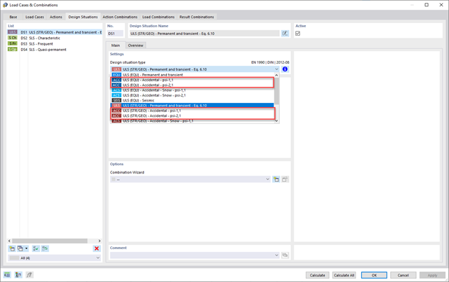
Do your structures also have to withstand unusual conditions? Then select the "accidental" design situation. Here, accidental actions such as earthquake, explosion loads, collisions, and many others, are considered automatically. Furthermore, when using German standards, you can select the "Accidental - Snow" design situation to consider the "North German Plain" automatically as well.
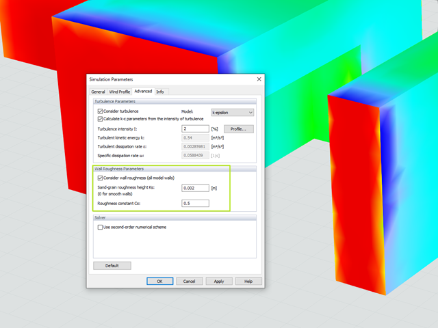
Utilize the RWIND Simulation program to consider a surface roughness of the model surface by applying a modified wall boundary condition. The numerical model is based on the assumption that grains with a certain diameter are arranged homogeneously on the model surface, similar to sandpaper. The grain diameter is described with the parameter Ks and the distribution with the parameter Cs. By considering the wall roughness, the numerical flow simulation can capture reality more closely.
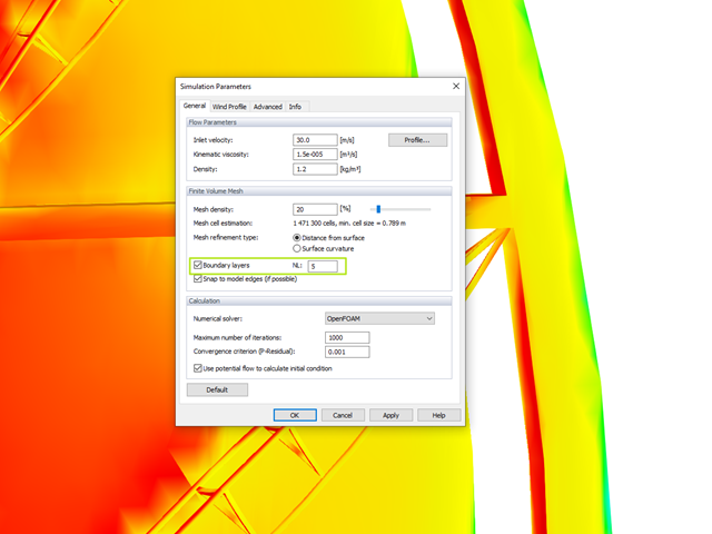
The meshing algorithm of RWIND Simulation uses the boundary layer option to mesh the area near the model surface with a voluminous layer mesh. The number of layers is controlled by a user-defined parameter.
This fine mesh in the area of the model surface helps to represent the wind velocity close to the surface.
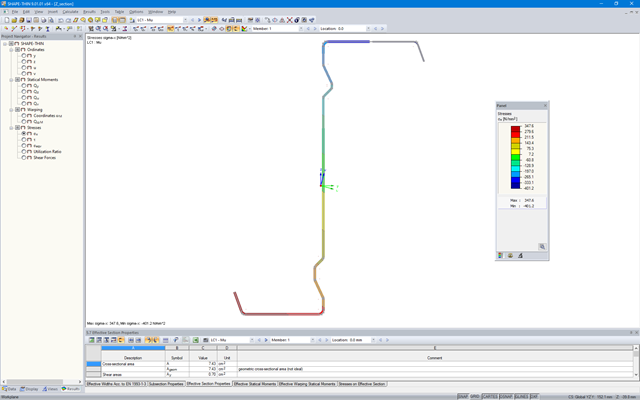
SHAPE‑THIN determines the effective cross-sections according to EN 1993‑1‑3 and EN 1993‑1‑5 for cold-formed sections. You can optionally check the geometric conditions for the applicability of the standard specified in EN 1993‑1‑3, Section 5.2.
The effects of local plate buckling are considered according to the method of reduced widths, and the possible buckling of stiffeners (instability) is considered for stiffened sections according to EN 1993‑1‑3, Section 5.5.
As an option, you can perform an iterative calculation to optimize the effective cross-section.
You can display the effective cross-sections graphically.
Read more about designing cold-formed sections with SHAPE-THIN and RF-/STEEL Cold-Formed Sections in the technical article "Design of Thin-Walled, Cold-Formed C-Section According to EN 1993‑1‑3".
Design of Thin-Walled, Cold-Formed C-Section According to EN 1993-1-3 More about RF-/STEEL Cold-Formed Sections
- 3D incompressible wind flow analysis with OpenFOAM® software package
- Direct model import from RFEM or RSTAB including neighboring and terrain models (3DS, IFC, STEP files)
- Model design via STL or VTP files independent of RFEM or RSTAB
- Simple model changes using Drag and Drop and graphical adjustment assistance
- Automatic corrections of the model topology with shrink wrap networks
- Option to add objects from the environment (buildings, terrain ...)
- Wind load determined over the height of the building, depending on standard-specific parameters (velocity, turbulence intensity)
- K-epsilon and K-omega turbulence models
- Automatic mesh generation adjusted to the selected depth of detail
- Parallel calculation with optimal utilization of the capacity of multicore computers
- Results in just minutes for low-resolution simulations (up to 1 million cells)
- Results within a few hours for simulations with medium/high resolution (1‑10 million cells)
- Graphical display of results on the Clipper/Slicer planes (scalar and vector fields)
- Graphical display of streamlines
- Streamline animation (optional video creation)
- Definition of point and line probes
- Display of aerodynamic pressure coefficients
- Graphical display of turbulence properties in the wind field
- Optional meshing using the boundary layer option for the area near the model surface
- Consideration of rough model surfaces possible
- Optional use of a seond-order numerical Order
- Multilingual user interface (for example, German, English, Spanish, French)
- Documentation possible in the RFEM and RSTAB printout report
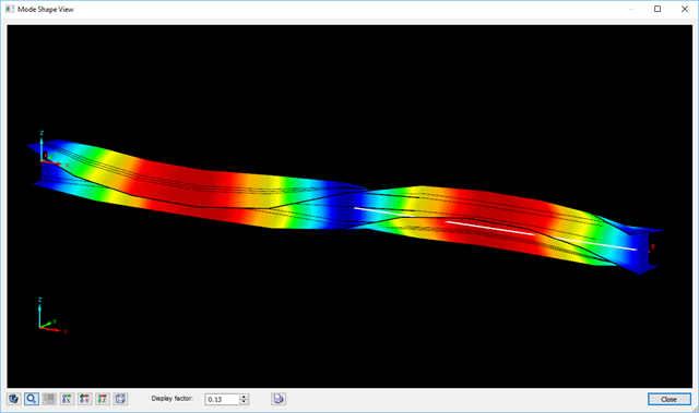
The determination of the critical buckling moment is carried out in RF-/STEEL AISC by using the eigenvalue solver which allows an exact determination of the critical buckling load.
The eigenvalue solver shows a display window of the eigenvalue graphics, which enables checking of the boundary conditions.
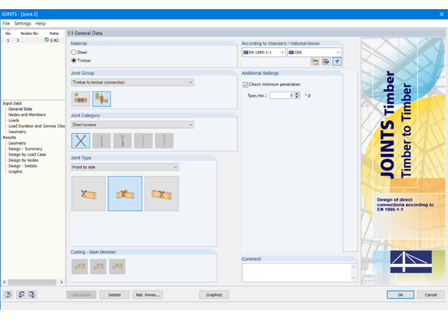
First, select the joint type and the design standard.
The connected members are imported from the RFEM/RSTAB model. The add-on module automatically checks if all geometry conditions are fulfilled.
In addition, the loads are imported automatically from RFEM/RSTAB. In the Geometry window, you can specify the screw parameters (diameter, length, angle, and so on).
.png?mw=640&hash=8cfd0c4bd093c03de543d147ffbf6f5c9250634a)
- User-defined time diagrams as a function of time, in tabular form, or as harmonic loads
- Combination of the time diagrams with RFEM/RSTAB load cases or combinations (enables definition of nodal, member, and surface loads, as well as free and generated loads varying over time)
- Combination of several independent excitation functions
- Nonlinear time history analysis with the implicit Newmark analysis (RFEM only) or the explicit analysis
- Structural damping using Rayleigh damping coefficients or Lehr's damping
- Direct import of initial deformations from a load case or combination (RFEM only)
- Stiffness modifications as initial conditions; for example, axial force effect, deactivated members (RSTAB only)
- Graphical display of results in a time history diagram
- Export of results in user-defined time steps or as an envelope
.png?mw=640&hash=688fdfc8af4828c08e9851cddb103a1e86cb899a)
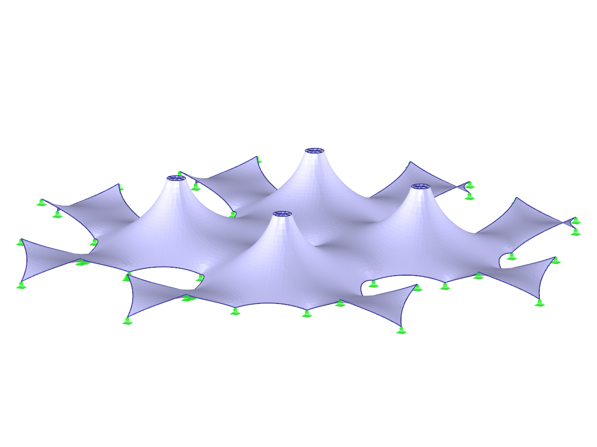
- Form-finding of:
- tension-loaded membrane and cable structures
- compression-loaded shell and beam structures
- mixed tension- and compression-loaded structures
- Consideration of gas chambers between surfaces
- Interaction with supporting structure (substructure design according to various standards)
- Surfaces as a 2D and members as a 1D element
- Definition of different prestress conditions for surfaces (membranes and shells)
- Definition of forces or geometrical requirements for members (cables and beams)
- Consideration of individual loads (self‑weight, inner pressure, and so on) in the form‑finding process
- Temporary support definitions for the form-finding process
- Automatic preliminary form-finding of membrane surfaces (more information...)
- Definition of isotropic or orthotropic material for structural analysis
- Optional definition of free polygon loads
- Transformation of form‑found shape elements into NURBS surface elements
- Possibility of combined form-finding by integration of preliminary form-finding
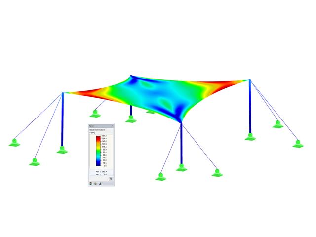
- Graphical evaluation of the new form using colored coordinates and inclination plots
- Complete documentation of the calculation including user-defined adaptive evaluation figures
- Optional export of the FE mesh as a DXF or Excel file
The nonlinear calculation adopts the real mesh geometry of planar, buckled, simple curved, or double curved surface components from the selected cutting pattern and flattens this surface component in compliance with the minimization of distortion energy, assuming defined material behavior.
In simplified terms, this method attempts to compress the mesh geometry in a press, assuming frictionless contact, and to find the state in which the stresses from flattening in the component are in equilibrium in the plane. This way, minimum energy and optimum accuracy of the cutting pattern are achieved. Compensation for warp and weft as well as compensation for boundary lines are considered. Then, the defined allowances on boundary lines are applied to the resulting planar surface geometry.
Features:
- Minimization of distortion energy in the flattening process for very accurate cutting patterns
- Application for almost all mesh arrangements
- Recognition of adjacent cutting pattern definitions to keep the same length
- Mesh application for main calculation
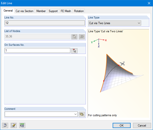
RF-CUTTING-PATTERN is activated by selecting the respective option in the Options tab in General Data of any RFEM model. After activating the add‑on module, a new object, "Cutting Patterns", is displayed under Model Data. If the membrane surface distribution for cutting in the basic position is too large, you can divide the surface by cutting lines (line types "Cut via Two Lines" or "Cut via Section") in the corresponding partial strips.
Then you can define the individual entries for each cutting pattern using the "Cutting Pattern" object. Here you can set boundary lines, compensations, and allowances.
Steps of the working sequence:
- Creation of cutting lines
- Creation of the pattern by selecting its boundary lines or using a semi‑automatic generator
- Free selection of warp and weft orientation by entering an angle
- Application of compensation values
- Optional definition of different compensations for boundary lines
- Different allowances (welding, boundary line)
- Preliminary representation of the cutting pattern in the graphic window at the side without starting the main nonlinear calculation
- Planar and geodesic cutting lines
- Flattening of double-curved surface parts of tensioned membranes or pneumatic cushions
- Definition of cutting patterns by using boundary lines which are not required to be connected
- Sophisticated flattening based on the minimum energy theory
- Welding and boundary allowances
- Uniform or linear compensation in warp and weft direction
- Possibility of different compensations for boundary lines
- Adaptable data organisation (any additional modification of input data is considered up to the final "weld")
- Graphical display of cutting patterns
- Statistical information about each cutting pattern (width, length, size)
- Option to automatically generate cutting patterns from cells