
The modal relevance factor (MRF) can help you to assess to which extent specific elements participate in a specific mode shape. The calculation is based on the relative elastic deformation energy of each individual member.
The MRF can be used to distinguish between local and global mode shapes. If multiple individual members show significant MRF (for example, > 20%), the instability of the entire structure or a substructure is very likely. On the other hand, if the sum of all MRFs for an eigenmode is around 100%, a local stability phenomenon (for example, buckling of a single bar) can be expected.
Furthermore, the MRF can be used to determine critical loads and equivalent buckling lengths of certain members (for example, for stability design). Mode shapes for which a specific member has small MRF values (for example, < 20%) can be neglected in this context.
The MRF is displayed by mode shape in the result table under Stability Analysis → Results by Members → Effective Lengths and Critical Loads.
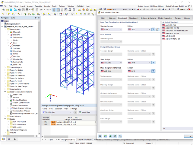
The design of cold-formed steel members according to the AISI S100-16 / CSA S136-16 is available in RFEM 6. Design can be accessed by selecting “AISC 360” or “CSA S16” as the standard in the Steel Design Add-on. “AISI S100” or “CSA S136” is then automatically selected for the cold-formed design.
RFEM applies the Direct Strength Method (DSM) to calculate the elastic buckling load of the member. The Direct Strength Method offers two types of solutions, numerical (Finite Strip Method) and analytical (Specification). The FSM signature curve and buckling shapes can be viewed under Sections.
.png?mw=640&hash=55038d2a1591f62179796666cb9b2fede0274e19)
A graphical and tabular output of the results for deformations, stresses, and strains helps you when determining the soil solids. To achieve this, use the special filter criteria for targeted selection of results.
The program doesn't leave you alone with the results. If you want to graphically evaluate the results in the soil solids, you can use the guide objects. For example, you can define clipping planes. This allows you to view the corresponding results in any plane of the soil solid.
And not just that. The utilization of result sections and clipping boxes facilitates the precise graphical analysis of the soil solid.
You already know that it is possible to model and analyze a soil and a structure in the entire model. As a result, you have explicitly taken into account the soil-structure interaction. By modifying a component, you achieve the immediate correct consideration in the analysis as well as in the results for the entire system of the soil and structure.

Are you ready for the evaluation? Use the calculation diagrams, which show the distribution of a specific result during the calculation.
You can freely define the layout of the vertical and horizontal axes of the calculation diagram. This allows you, for example, to consider the settlement distribution of a certain node, depending on the load.

Your data are always documented in a multilingual printout report. You can adjust the content at any time and save it as a template. You can also add graphics, texts, MathML formulas, and PDF documents to your report with just a few clicks.

Enter and model a soil solid directly in RFEM. You can combine the soil material models with all common RFEM add-ons.
This allows you to easily analyze the entire models with a complete representation of the soil-structure interaction.
All parameters required for the calculation are automatically determined from the material data that you have entered. The program then generates the stress-strain curves for each FE element.

Did you know? You can enter the soil layers that you have obtained from the subsoil expertises done in the locations into the program in the form of soil samples. Assign the explored soil materials, including their material properties, to the layers.
For the definition of the samples, you can enter the data in tables as well as in the respective editing dialog box. Furthermore, you can also specify the groundwater level in the soil samples.

The soil solids that you want to analyze are summarized in soil massifs.
Use the soil samples as a basis for a definition of the respective soil massif. This way, the program allows for user-friendly generation of the massif, including the automatic determination of the layer interfaces from the sample data, as well as the groundwater level and the boundary surface supports.
Soil massifs provide you with the option to specify a target FE mesh size independently of the global setting for the rest of the structure. You can thus consider the various requirements of the building and soil in the entire model.
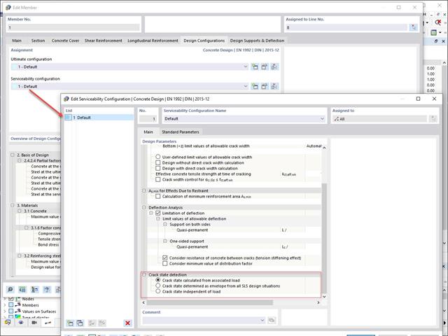
Various design parameters of the cross-sections can be adjusted in the serviceability limit state configuration. The applied cross-section condition for the deformation and crack width analysis can be controlled there.
For this, the following settings can be activated:
- Crack state calculated from associated load
- Crack state determined as an envelope from all SLS design situations
- Cracked state of cross-section - independent of load

Do you want to model and analyze the behavior of a soil solid? To ensure this, special suitable material models have been implemented in RFEM.
You can use the modified Mohr-Coulomb model with a linear-elastic ideal-plastic model or a nonlinear elastic model with an oedometric stress-strain relation. The limit criterion, which describes the transition from the elastic area to that of the plastic flow, is defined according to Mohr-Coulomb.
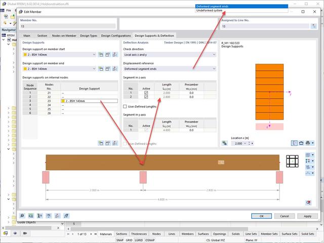
In the "Deflection and Design Support" tab under "Edit Member", the members can be clearly segmented using optimized input windows. Depending on the supports, the deformation limits for cantilever beams or single-span beams are used automatically.
By defining the design support in the corresponding direction at the member start, member end, and intermediate nodes, the program automatically recognizes the segments and segment lengths to which the allowable deformation is related. It also automatically detects whether it is a beam or a cantilever due to the defined design supports. The manual assignment, as in the previous versions (RFEM 5), is no longer necessary.
The "User-Defined Lengths" option allows you to modify the reference lengths in the table. The corresponding segment length is always used by default. If the reference length deviates from the segment length (for example, in the case of curved members), it can be adjusted.
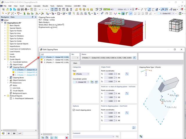
This feature also contributes to the clearly-arranged display of your results. Clipping planes are intersecting planes that you can place freely throughout the model. The zone in front of or behind the plane is consequently hidden in the display. This way, you can clearly and simply show the results in an intersection or a solid, for example.
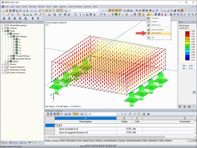
The results of solid stresses can be displayed as colored 3D points in the finite elements.

Compared to the RF‑SOILIN add-on module (RFEM‑5), the following new features have been added to the Geotechnical Analysis add-on for RFEM 6:
- Creation of the layered soil as a 3D model from the entirety of the defined soil samples
- Recognized material law according to Mohr-Coulomb for soil simulation
- Graphical and tabular output of stresses and strains at any depth of the soil
- Optimal consideration of the soil-structure interaction on the basis of an overall model

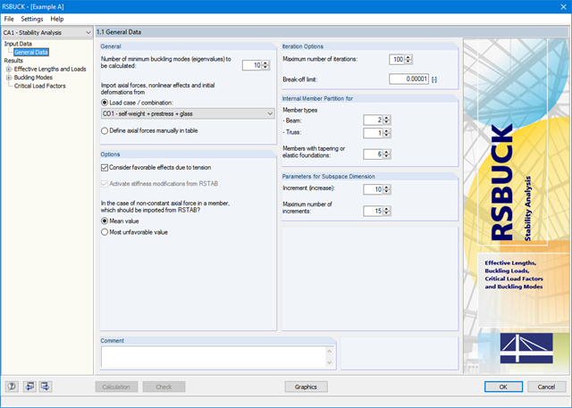
Compared to the RF‑/STABILITY (RFEM 5) and RSBUCK (RSTAB 8) add-on modules, the following new features have been added to the Structure Stability add-on for RFEM 6 / RSTAB 9:
- Activation as a property of a load case or a load combination
- Automated activation of the stability calculation via combination wizards for several load situations in one step
- Incremental load increase with user-defined termination criteria
- Modification of the mode shape normalization without recalculation
- Result tables with filter option

- Calculation of models consisting of member, shell, and solid elements
- Nonlinear stability analysis
- Optional consideration of axial forces from initial prestress
- Four equation solvers for an efficient calculation of various structural models
- Optional consideration of stiffness modifications in RFEM/RSTAB
- Determination of a stability mode greater than the user-defined load increment factor (Shift method)
- Optional determination of the mode shapes of unstable models (to identify the cause of instability)
- Visualization of the stability mode
- Basis for determining imperfection
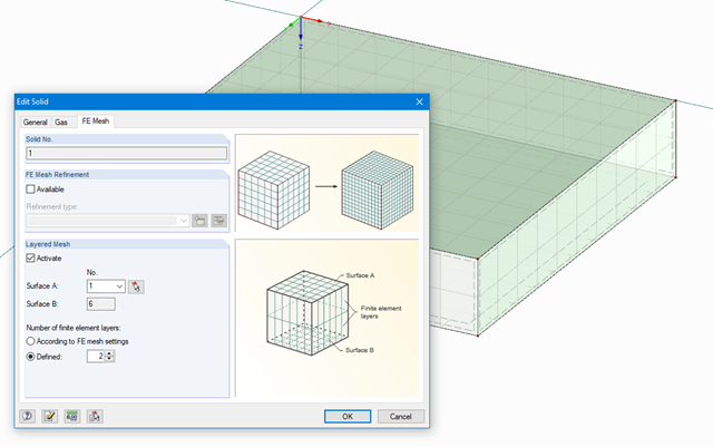
The stiffness of gas given by the ideal gas law pV = nRT can be considered in the nonlinear dynamic analysis.
The calculation of gas is available for accelerograms and time diagrams for both the explicit analysis and the nonlinear implicit Newmark analysis. To determine the gas behavior correctly, at least two FE layers for gas solids should be defined.
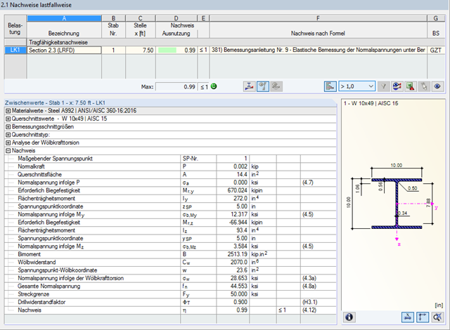
Due to the integrated RF-/STEEL Warping Torsion module extension, it is possible to perform the design according to Design Guide 9 in RF-/STEEL AISC.
The calculation is performed with 7 degrees of freedom according to the warping torsion theory and enables a realistic stability design, including consideration of torsion.
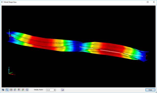
The determination of the critical buckling moment is carried out in RF-/STEEL AISC by using the eigenvalue solver which allows an exact determination of the critical buckling load.
The eigenvalue solver shows a display window of the eigenvalue graphics, which enables checking of the boundary conditions.
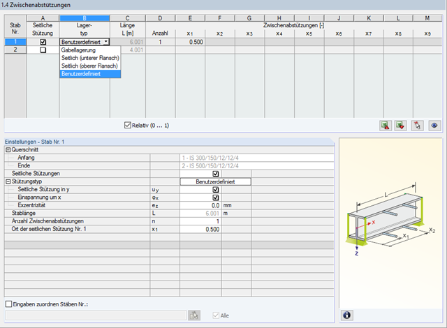
In STEEL AISC, it is possible to consider lateral intermediate supports at any location. For example, it is possible to stabilize only the upper flange.
Furthermore, user-defined lateral intermediate supports can be assigned; for example, single rotational springs and translational springs at any location at the cross-section.
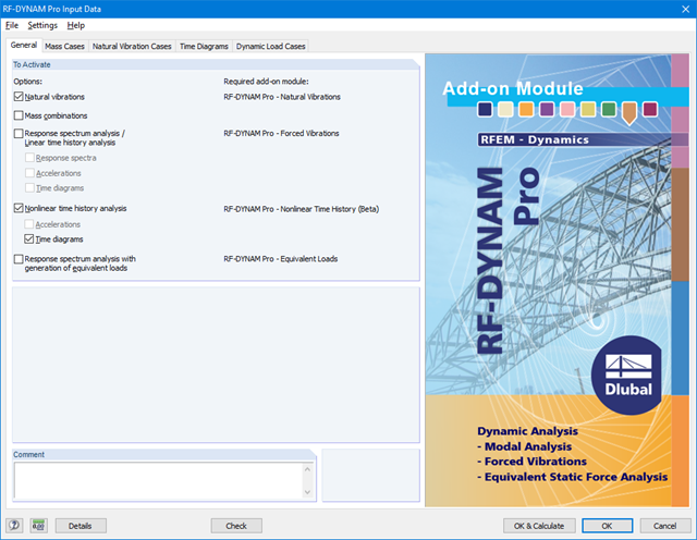
RF-/DYNAM Pro - Nonlinear Time History is integrated in the structure of RF‑/DYNAM Pro - Forced Vibrations and extended by two nonlinear analysis methods (one nonlinear analysis in RSTAB).
Force-time diagrams can be entered as transient, periodic, or as a function of time. Dynamic load cases combine the time diagrams with the static load cases, which provides high flexibility. Furthermore, it is possible to define time steps for the calculation, structural damping, and export options in the dynamic load cases.

- Nonlinear member types, such as tension and compression members or cables
- Member nonlinearities, such as failure, tearing, yielding under tension or compression
- Support nonlinearities, such as failure, friction, diagram, and partial activity
- Release nonlinearities, such as friction, partial activity, diagram, and fixed if positive or negative internal forces
.png?mw=640&hash=8cfd0c4bd093c03de543d147ffbf6f5c9250634a)
- User-defined time diagrams as a function of time, in tabular form, or as harmonic loads
- Combination of the time diagrams with RFEM/RSTAB load cases or combinations (enables definition of nodal, member, and surface loads, as well as free and generated loads varying over time)
- Combination of several independent excitation functions
- Nonlinear time history analysis with the implicit Newmark analysis (RFEM only) or the explicit analysis
- Structural damping using Rayleigh damping coefficients or Lehr's damping
- Direct import of initial deformations from a load case or combination (RFEM only)
- Stiffness modifications as initial conditions; for example, axial force effect, deactivated members (RSTAB only)
- Graphical display of results in a time history diagram
- Export of results in user-defined time steps or as an envelope
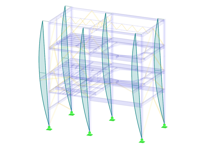
The add-on module evaluates the pre-deformation of a load case as well as mode shapes of stability or dynamic analysis. Based on this initial deformation, it is possible either to pre-deform the structure or to create a load case with equivalent imperfections of members.
The pre-deformed initial model is useful especially for structures consisting of surface and solid elements (RFEM) as well as members. It is necessary to specify only the maximum value to which the deformation is to be scaled. All FE or model nodes will be scaled with regard to the initial deformation.
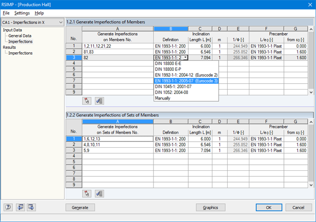
Equivalent imperfections are particularly useful for beam structures. You can define inclinations and precambers of members and sets of members in the additional window. They can be generated automatically, according to standards, or defined manually. The following standards are available:
-
 EN 1992:2004
 -
EN 1993:2005
-
 DIN 18800:1990-11
 -
DIN 1045-1:2001-07
-
DIN 1052:2004-08
Only the imperfection resulting from the initial deformation on the relevant member is applied. In addition, you can consider the reduction factors. This way, it is possible to apply the imperfection efficiently.
- Creation of a pre-deformed FE mesh in RFEM
- Generation of equivalent imperfections of members as equivalent loads, considering
- the reduction factors αu and αm (Eurocode)
- the precamber rises according to buckling stress curves
- Deformation of the structure due to nodal displacement
- Generation of imperfections in accordance with:
- the load case deformations
- the buckling shapes from RF-STABILITY/RSBUCK
- Equivalent imperfections on members and sets of members (for example, columns consisting of several members)
- Visualization of generated imperfection modes
- Automatic import of structural data and boundary conditions from RSTAB
- Optional consideration of favorable effects due to tension
- Import of axial forces from RSTAB load cases or user-defined specifications for member
- Member-wise output of effective lengths L about weak and strong axis with corresponding effective length factors β
- Results by member listing standardized buckling modes
- Results of critical load factors regarding buckling case for entire structure
- Graphics and animated visualization of buckling modes on the rendered model
- Identification of members free of compression forces
- Optional transfer of the effective lengths to other RSTAB design modules for equivalent member designs according to standards
- Optional export of buckling mode geometry to the RSIMP add-on module in order to create RSTAB imperfections
- Direct data export to MS Excel
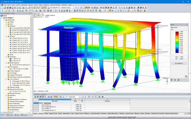
The first results presented are the critical load factors. This allows for an evaluation of stability risks. For member models, the effective lengths and critical loads of the members are output in tabular form.
In the next result windows, you can check the normalized eigenvalues sorted by node, member, and surface. The eigenvalue graphic allows for evaluation of the buckling behavior. The graphical display makes it easier to take countermeasures.
Several methods are available for the eigenvalue analysis:
- Direct Methods
- The direct methods (Lanczos, roots of characteristic polynomial, subspace iteration method) are suitable for small to medium-sized models. These fast methods for equation solvers benefit from a lot of the computer memory (RAM). 64-bit systems use more memory so that even bigger structural systems can be calculated quickly.
- ICG iteration method (Incomplete Conjugate Gradient)
- This method requires only a small amount of memory. Eigenvalues are determined one after the other. It can be used to calculate large structural systems with few eigenvalues.
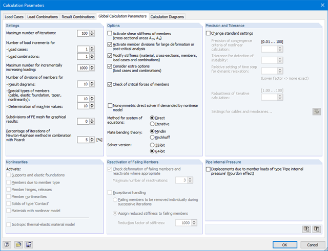
The RF-STABILITY add-on module can also perform the non-linear stability analysis. Also for nonlinear structures, results close to reality are provided. The critical load factor is determined by gradually increasing the loads of the underlying load case until the instability is reached. The load increment takes into account nonlinearities such as failing members, supports and foundations, and material nonlinearities.
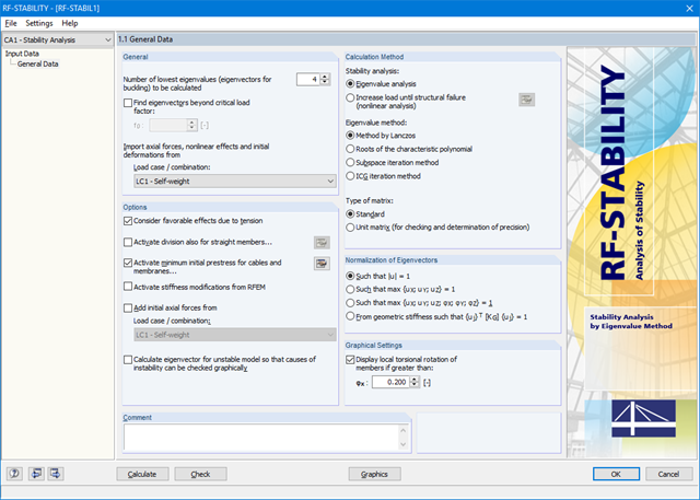
First of all, it is necessary to select a load case or combination whose axial forces are to be used in the stability analysis. It is possible to define another load case to, for example, For example, you have to consider an initial prestress.
Then, you can select the linear or non-linear analysis to be performed. Depending on the application, you can use a direct calculation method, such as according to Lanczos or the ICG iteration method. Members not integrated in surfaces are usually displayed as member elements with two FE nodes. It is not possible to determine the local buckling of single members on these elements. Therefore, you have the option to divide members automatically.