
- 002161
- General
- Optimization & Cost / CO2 Emission Estimation for RFEM 6
- Optimization & Cost / CO2 Emission Estimation for RSTAB 9
Both optimization methods have one thing in common. At the end of the process, they provide you with a list of model mutations from the stored data. Here you can find the details of the controlling optimization result and the associated value assignment of the optimization parameters. This list is organized in descending order. You can find the assumed best solution shown in the first line. For this, the optimization result with its determined value assignment is closest to the optimization criterion. All add-on results have a utilization < 1. Furthermore, once the analysis is completed, the program will adjust the value assignment to that of the optimal solution for the optimization parameters in the global parameter list.
In the material dialog boxes, you can find the additional tabs "Cost Estimation" and "Estimation of CO2 Emissions". They show you the individual estimated sums of the assigned members, surfaces, and solids per unit weight, volume, and area. Furthermore, these tabs show the total cost and emission of all assigned materials. This gives you a good overview of your project.

In the Modal Analysis add-on, you have the option to automatically increase the sought eigenvalues until reaching a defined effective modal mass factor. All translational directions activated as masses for the modal analysis are taken into account.
Thus, it is possible to easily calculate the required 90% of the effective modal mass for the response spectrum method.
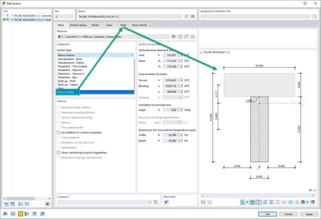
In the Construction Stages Analysis (CSA) add-on, you can use built-up cross-sections by means of what are known as phase sections. This allows you to activate and deactivate the parts of the "Parametric - Massive II" section type throughout the construction stages.

You have several options available to define masses for a modal analysis. While the masses due to self-weight are considered automatically, you can consider the loads and masses directly in a load case of the modal analysis type. Do you need more options? Select whether to consider full loads as masses, load components in the global Z-direction, or only the load components in the direction of gravity.
The program offers you an additional or alternative option for importing masses: A manual definition of load combinations as of which are the masses considered in the modal analysis. Have you selected a design standard? You can then create a design situation with the Seismic Mass combination type. Thus, the program automatically calculates a mass situation for the modal analysis according to the preferred design standard. In other words: The program creates a load combination on the basis of the preset combination coefficients for the selected standard. This contains the masses used for the modal analysis.

For a response spectrum analysis of building models, you can display the sensitivity coefficients for the horizontal directions by story.
These key figures allow you to interpret the sensitivity to stability effects.

- 002109
- General
- Optimization & Cost / CO2 Emission Estimation for RFEM 6
- Optimization & Cost / CO2 Emission Estimation for RSTAB 9
Did you know? The structural optimization in the programs RFEM and RSTAB is a completion of the parametric input. It is a parallel process beside the actual model calculation with all its regular calculation and design definitions. The add-on assumes that your model or block is built with a parametric context and is controlled in its entirety by global control parameters of the "optimization" type. Therefore, these control parameters have a lower and upper limit and a step size to delimit the optimization range. If you want to find optimal values for the control parameters, you have to specify an optimization criterion (for example, minimum weight) with the selection of an optimization method (for example, particle swarm optimization).
You can already find the cost and CO2 emission estimation in the material definitions. You can activate both options individually in each material definition. The estimation is based on a unit for unit cost or unit emission for members, surfaces, and solids. In this case, you can select whether to specify the units by weight, volume, or area.

- 002108
- General
- Optimization & Cost / CO2 Emission Estimation for RFEM 6
- Optimization & Cost / CO2 Emission Estimation for RSTAB 9
- Artificial intelligence technology (AI): Particle swarm optimization (PSO)
- Structure optimization according to the minimum weight or deformation
- Use of any number of optimization parameters
- Specification of variable ranges
- Optimization of cross-sections and materials
- Parameter definition types
- Optimization | Ascending or Optimization | Descending
- Application of parametric models and blocks
- Code-based JavaScript parametrization of blocks
- Optimization taking into account the design results
- Tabular display of the best model mutations
- Real-time display of the model mutations in the optimization process
- Model cost estimation by specifying unit prices
- Determination of the global warming potential GWP when realizing the model by estimating the CO2 equivalent
- Specification of weight-, volume-, and area-based units (price and CO2e)

In RFEM, you can use these three powerful eigenvalue solvers:
- Root of Characteristic Polynomial
- Method by Lanczos
- Subspace Iteration
RSTAB, on the other hand, provides you with these two eigenvalue solvers:
- Subspace Iteration
- Shifted inverse power method
The selection of the eigenvalue solver depends primarily on your model size.

- 002110
- General
- Optimization & Cost / CO2 Emission Estimation for RFEM 6
- Optimization & Cost / CO2 Emission Estimation for RSTAB 9
There are two methods that you can use for the optimization process, with which you can find optimal parameter values according to a weight or deformation criterion.
The most efficient method with the littlest calculation time is the near-natural particle swarm optimization (PSO). Have you heard or read about it? This artificial intelligence (AI) technology has a strong analogy to the behavior of flocks of animals, looking for a resting place. In such swarms, you can find many individuals (cf. optimization solution - for example, weight) who like to stay in a group and follow the group movement. Let's assume that each individual swarm member has a need to rest at an optimal resting place (cf. best solution - for example, lowest weight). This need increases as the resting place is approached. Thus, the swarm behavior is also influenced by the properties of the space (cf. result diagram).
Why the excursion into biology? Quite simply – the PSO process in RFEM or RSTAB proceeds in a similar way. The calculation run starts with an optimization result from a random assignment of the parameters to be optimized. It repeatedly determines new optimization results with varied parameter values, which are based on the experience of the previously performed model mutations. The process continues until the specified number of possible model mutations is reached.
As an alternative to this method, the program also offers you a batch processing method. This method attempts to check all possible model mutations by randomly specifying the values for the optimization parameters until a predetermined number of possible model mutations is reached.
After calculating a model mutation, both variants also check the respective activated design results of the add-ons. Furthermore, they save the variant with the corresponding optimization result and value assignment of the optimization parameters if the utilization is < 1.
You can determine the estimated total costs and emission from the respective sums of the individual materials. The sums of the materials are composed of the weight-based, volume-based, and area-based partial sums of the member, surface, and solid elements.

Have you created the entire structure in RFEM? Very well, now you can assign the individual structural components and load cases to the corresponding construction stages. In each construction stage, you can modify release definitions of members and supports, for example.
You can thus model structural modifications, such as those that occur when bridge girders are successively grouted or when columns are settled. Then, assign the load cases created in RFEM to the construction stages as permanent or non-permanent loads.
Did you know that The combinatorics allows you to superimpose the permanent and non-permanent loads in load combinations. In this way, it is possible for you to determine the maximum internal forces of different crane positions or to consider temporary mounting loads available in one construction stage only.

- Automatic consideration of masses from self-weight
- Direct import of masses from load cases or load combinations
- Optional definition of additional masses (nodal, linear, or surface masses, as well as inertia masses) directly in the load cases
- Optional neglect of masses (for example, mass of foundations)
- Combination of masses in different load cases and load combinations
- Preset combination coefficients for various standards (EC 8, SIA 261, ASCE 7,...)
- Optional import of initial states (for example, to consider prestress and imperfection)
- Structure Modification
- Consideration of failed supports or members/surfaces/solids
- Definition of several modal analyses (for example, to analyze different masses or stiffness modifications)
- Selection of mass matrix type (diagonal matrix, consistent matrix, unit matrix), including user-defined specification of translational and rotational degrees of freedom
- Methods for determining the number of mode shapes (user-defined, automatic - to reach effective modal mass factors, automatic - to reach the maximum natural frequency - only available in RSTAB)
- Determination of mode shapes and masses in nodes or FE mesh points
- Results of eigenvalue, angular frequency, natural frequency, and period
- Output of modal masses, effective modal masses, modal mass factors, and participation factors
- Masses in mesh points displayed in tables and graphics
- Visualization and animation of mode shapes
- Various scaling options for mode shapes
- Documentation of numerical and graphical results in printout report
- Simple definition of construction stages in the RFEM structure including visualization
- Adding, removing, modifying, and reactivating member, surface, and solid elements and their properties (for example, member and line hinges, degrees of freedom for supports, and so on)
- Automatic and manual combinatorics with load combinations in the individual construction stages (for example, to consider mounting loads, mounting cranes, and other loads)
- Consideration of nonlinear effects such as tension member failure or nonlinear supports
- Interaction with other add-ons, such as Nonlinear Material Behavior, Structure Stability, Form-Firnding, and so on.
- Display of results numerically and graphically for individual construction stages
- Detailed printout report with documentation of all structural and load data for each construction stage

If there are geometry differences arising between the ideal and the deformed structural system from the previous construction stage, they are compared in the program. The next construction stage is built on top of the stressed system from the previous construction stage. This calculation is nonlinear.

In the modal analysis settings, you have to enter all data that are necessary for the determination of the natural frequencies. These are, for example, mass shapes and eigenvalue solvers.
The Modal Analysis add-on determines the lowest eigenvalues of the structure. Either you adjust the number of eigenvalues or let them determined automatically. Thus, you should reach either effective modal mass factors or maximum natural frequencies. Masses are imported directly from load cases and load combinations. In this case, you have the option to consider the total mass, load components in the global Z-direction, or only the load component in the direction of gravity.
You can manually define additional masses at nodes, lines, members, or surfaces. Furthermore, you can influence the stiffness matrix by importing axial forces or stiffness modifications of a load case or load combination.
Compared to the RF‑/STAGES add-on module (RFEM 5), the following new features have been added to the Construction Stages Analysis (CSA) add-on for RFEM 6:
- Consideration of construction stages at RFEM level
- Integration of the construction stage analysis into the combinatorics in RFEM
- Additional structural elements, such as line hinges, are supported
- Analysis of alternative construction processes in a model
- Reactivation of elements

Was the calculation successful? Now you can view the results of the individual construction stages graphically and in tables in RFEM. Moreover, RFEM allows you to consider the construction stages in the combinatorics and include it in further design.

Do you want to consider other loads as masses in addition to the static loads? The program allows that for nodal, member, line and surface loads. For this, you need to select the Mass load type when defining the load of interest. Define a mass or mass components in the X, Y, and Z directions for such loads. For nodal masses, you have an additional option to also specify moments of inertia X, Y, and Z in order to model more complex mass points.

The Dlubal structural analysis software does a lot of work for you. The input parameters, which are relevant for the selected standards, are suggested by the program in accordance with the rules. Furthermore, you can enter response spectra manually.
Load cases of the type Response Spectrum Analysis define the direction in which response spectra act and which eigenvalues of the structure are relevant for the analysis. In the spectral analysis settings, you can define details for the combination rules, damping (if applicable), and zero-period acceleration (ZPA).

As soon as the program has completed the calculation, the eigenvalues, natural frequencies and periods are listed. These result windows are integrated in the main program RFEM/RSTAB. You can find all mode shapes of the structure in tables and also have an option to display them graphically and to animate them.
All result tables and graphics are part of the RFEM/RSTAB printout report. In this way, you can ensure clearly arranged documentation. You can also export the tables to MS Excel.

It is often necessary to neglect masses. This is particularly the case when you want to use the output of the modal analysis for the seismic analysis. For this, 90% of the effective modal mass in each direction is required for the calculation. So you can neglect the mass in all fixed nodal and line supports. The program automatically deactivates the associated masses for you.
You can also manually select the objects whose masses are to be neglected for the modal analysis. We have shown the latter in the image for a better view. A user-defined selection is made the and the objects with their associated mass components are selected to neglect the masses.

You can already see it in the image: Imperfections can also be taken into account when defining a modal analysis load case. The imperfection types that you can use in the modal analysis are notional loads from load case, initial sway via table, static deformation, buckling mode, dynamic mode shape, and group of imperfection cases.

When defining the input data for the modal analysis load case, you can consider a load case whose stiffnesses represent the initial position for the modal analysis. How do you do that? As shown in the image, select the "Consider initial state from" option. Now, open the "Initial State Settings" dialog box and define the type Stiffness as the initial state. In this load case, as of which is the initial state taken into account, you can consider the stiffness of the structural system when the tension members fail. The purpose of all of this: The stiffness from this load case is considered in the modal analysis. Thus, you obtain a clearly flexible system.

Compared to the RF‑/DYNAM Pro - Natural Vibrations add-on module (RFEM 5 / RSTAB 8), the following new features have been added to the Modal Analysis add-on for RFEM 6 / RSTAB 9:
- Preset combination coefficients for various standards (EC 8, ASCE, and so on)
- Optional neglect of masses (for example, mass of foundations)
- Methods for determining the number of mode shapes (user-defined, automatic - to reach effective modal mass factors, automatic - to reach the maximum natural frequency)
- Output of modal masses, effective modal masses, modal mass factors, and participation factors
- Masses in mesh points displayed in tables and graphics
- Various scaling options for mode shapes in the Result navigator

The form-finding process gives you a structural model with active forces in the "prestress load case" This load case shows the displacement from the initial input position to the form-found geometry in the deformation results. In the force or stress-based results (member and surface internal forces, solid stresses, gas pressures, and so on), it clarifies the state for maintaining the found form. For the analysis of the shape geometry, the program offers you a two-dimensional contour line plot with the output of the absolute height and an inclination plot for the visualization of the slope situation.
Now, a further calculation and structural analysis of the entire model is performed. For this purpose, the program transfers the form-found geometry including the element-wise strains into a universally applicable initial state. You can now use it in the load cases and load combinations.

Did you know? You can easily define structural modifications in load cases of the Modal Analysis type. This allows you, for example, to individually adjust the stiffnesses of materials, cross-sections, members, surfaces, hinges, and supports. You can also modify stiffnesses for some design add-ons. Once you select the objects, their stiffness properties are adapted to the object type. In this way, you can define them in separate tabs.
Do you want to analyze the failure of an object (for example, a column) in the modal analysis? This is also possible without any problems. Simply switch to the Structure Modification window and deactivate the relevant objects.

The Ponding load type allows you to simulate rain actions on multi-curved surfaces, taking into account the displacements according to the large deformation analysis.
This numerical rainfall process examines the assigned surface geometry and determines which rainfall portions drain away and which rainfall portions accumulate in puddles (water pockets) on the surface. The puddle size then results in a corresponding vertical load for the structural analysis.
For example, you can use this feature in the analysis of approximately horizontal membrane roof geometries subjected to rain loading.
Go to Explanatory Video
Once you activate the Form-Finding add-on in the Base Data, a form-finding effect is assigned to the load cases with the load case category "Prestress" in conjunction with the form-finding loads from the member, surface, and solid load catalog. This is a prestress load case. It thus mutates into a form-finding analysis for the entire model with all member, surface, and solid elements defined in it. You reach the form-finding of the relevant member and membrane elements amid the overall model by using special form-finding loads and regular load definitions. These form-finding loads describe the expected state of deformation or force after the form-finding in the elements. The regular loads describe the external loading of the entire system.

The load cases of the type Response Spectrum Analysis contain the generated equivalent loads. First, the modal contributions have to be superimposed with the SRSS or CQC rule. In this case, you can use the signed results based on the dominant mode shape.
Afterwards, the directional components of earthquake actions are combined with the SRSS or the 100% / 30% rule.
Compared to the RF-/DYNAM Pro - Equivalent Loads add-on module (RFEM 5 / RSTAB 8), the following new features have been added to the Response Spectrum Analysis add-on for RFEM 6 / RSTAB 9:
- Response spectra of numerous standards (EN 1998, DIN 4149, IBC 2018, and so on)
- User-defined response spectra or those generated from accelerograms
- Direction-relative response spectrum approach
- Results are stored centrally in a load case with underlying levels to ensure clarity
- Accidental torsional actions can be taken into account automatically
- Automatic combinations of seismic loads with the other load cases for use in an accidental design situation

Compared to the RF-FORM-FINDING add-on module (RFEM 5), the following new features have been added to the Form-Finding add-on for RFEM 6:
- Specification of all form-finding load boundary conditions in one load case
- Storage of form-finding results as initial state for further model analysis
- Automatic assignment of the form-finding initial state via combination wizards to all load situations of a design situation
- Additional form-finding geometry boundary conditions for members (unstressed length, maximum vertical sag, low-point vertical sag)
- Additional form-finding load boundary conditions for members (maximum force in member, minimum force in member, horizontal tension component, tension at i-end, tension at j-end, minimum tension at i-end, minimum tension at j-end)
- Material types "Fabric" and "Foil" in material library
- Parallel form-findings in one model
- Simulation of sequentially building form-finding states in connection with the Construction Stages Analysis (CSA) add-on