
In the Stress-Strain Analysis add-on, you can define a component-dependent limit stress cycle and consider it for the design.
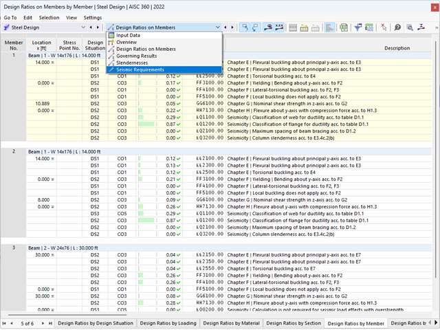
The seismic design result is categorized into two sections: member requirements and connection requirements.
The "Seismic Requirements" include the Required Flexural Strength and the Required Shear Strength of the beam-to-column connection for moment frames. They are listed in the ‘Moment Frame Connection by Member’ tab. For braced frames, the Required Connection Tensile Strength and the Required Connection Compressive Strength of the brace are listed in the ‘Brace Connection by Member’ tab.
The program provides the performed design checks in tables. The design check details clearly display the formulas and references to the standard.

Both optimization methods have one thing in common. At the end of the process, they provide you with a list of model mutations from the stored data. Here you can find the details of the controlling optimization result and the associated value assignment of the optimization parameters. This list is organized in descending order. You can find the assumed best solution shown in the first line. For this, the optimization result with its determined value assignment is closest to the optimization criterion. All add-on results have a utilization < 1. Furthermore, once the analysis is completed, the program will adjust the value assignment to that of the optimal solution for the optimization parameters in the global parameter list.
In the material dialog boxes, you can find the additional tabs "Cost Estimation" and "Estimation of CO2 Emissions". They show you the individual estimated sums of the assigned members, surfaces, and solids per unit weight, volume, and area. Furthermore, these tabs show the total cost and emission of all assigned materials. This gives you a good overview of your project.

In the Modal Analysis add-on, you have the option to automatically increase the sought eigenvalues until reaching a defined effective modal mass factor. All translational directions activated as masses for the modal analysis are taken into account.
Thus, it is possible to easily calculate the required 90% of the effective modal mass for the response spectrum method.

In the Geotechnical Analysis add-on, the Hoek-Brown material model is available. The model shows linear-elastic ideal-plastic material behavior. Its nonlinear strength criterion is the most common failure criterion for stone and rocks.
You can enter the material parameters using
- Rock parameters directly, or alternatively via
- GSI classification.
Detailed information about this material model and the definition of the input in RFEM can be found in the respective chapter Hoek-Brown Model of the online manual for the Geotechnical Analysis add-on.
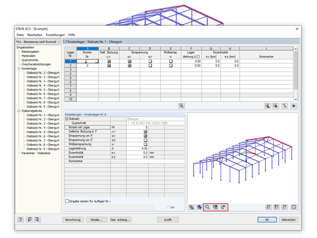
- For the design according to Eurocode 3, the parameters of the National Annexes (NA) are integrated for the following countries:
-
 DIN EN 1993-1-1/NA:2016-04 (Germany)
 -
 ÖNORM EN 1993-1-1/NA:2015-12 (Austria)
 -
 SN EN 1993-1-1/NA:2016-07 (Switzerland)
 -
 BDS EN 1993-1-1/NA:2015-10 (Bulgaria)
 -
 BS EN 1993-1-1/NA:2016-07 (United Kingdom)
 -
 CEN EN 1993-1-1/2015-06 (European Union)
 -
 CYS EN 1993-1-1/NA:2015-07 (Cyprus)
 -
 CZE EN 1993-1-1/NA:2016-06 (Czech Republic)
 -
 DS EN 1993-1-1/NA:2015-07 (Denmark)
 -
 ELOT EN 1993-1-1/NA:2017-01 (Greece)
 -
 EVS EN 1993-1-1/NA:2015-08 (Estonia)
 -
 HRN EN 1993-1-1/NA:2016-03 (Croatia)
 -
 I S. EN 1993-1-1/NA:2016-03 (Ireland)
 -
 ILNAS EN 1993-1-1/NA:2015-06 (Luxembourg)
 -
 IST EN 1993-1-1/NA:2015-11 (Iceland)
 -
 LST EN 1993-1-1/NA:2017-01 (Lithuania)
 -
 LVS EN 1993-1-1/NA:2015-10 (Latvia)
 -
 MS EN 1993-1-1/NA:2010-01 (Malaysia)
 -
 MSZ EN 1993-1-1/NA:2015-11 (Hungary)
 -
 NBN EN 1993-1-1/NA:2015-07 (Belgium)
 -
 NEN EN 1993-1-1/NA:2016-12 (Netherlands)
 -
 NF EN 1993-1-1/NA:2016-02 (France)
 -
 NP EN 1993-1-1/NA:2009-03 (Portugal)
 -
 NS EN 1993-1-1/NA:2015-09 (Norway)
 -
 PN EN 1993-1-1/NA:2015-08 (Poland)
 -
 SFS EN 1993-1-1/NA:2015-08 (Finland)
 -
 SIST EN 1993-1-1/NA:2016-09 (Slovenia)
 -
 SR EN 1993-1-1/NA:2016-04 (Romania)
 -
 SS EN 1993-1-1/NA:2019-05 (Singapore)
 -
 SS EN 1993-1-1/NA:2015-06 (Sweden)
 -
 STN EN 1993-1-1/NA:2015-10 (Slovakia)
 -
 TKP EN 1993-1-1/NA:2015-04 (Belarus)
 -
 UNE EN 1993-1-1/NA:2016-02 (Spain)
 -
 UNI EN 1993-1-1/NA:2015-08 (Italy)
-
- The design according to US standard AISC 360 includes analysis methods according to:
-
 Load and Resistance Factor Design (LRFD)
 -
Allowable Stress Design (ASD)
-
- Manual specification of critical component temperature or automatic determination of component temperature for desired duration
- A wide range of fire curves: standard temperature-time curve, external fire curve, hydrocarbon curve
- Manual adjustment of the essential coefficients for the determination of the steel temperature
- Consideration of hot-dip galvanizing of structural components for the determination of the steel temperature
- Results of a temperature-time diagram for the gas and steel temperature
- Fire protection cladding as a contour or a box cladding with temperature-independent materials can be considered when determining the temperature
- Design of members made of carbon steel or stainless steel
- Cross-section design checks and stability analyses (equivalent member method) according to EN 1993‑1‑2, Clause 4.2.3
- Design checks of the cross-sections of Class 4 according to EN 1993‑1‑2, Annex E.

Building stone on stone has a long tradition in construction. The Masonry Design add-on for RFEM allows you to design masonry using the finite element method. It was developed as part of the research project DDMaS - Digitizing the Design of Masonry Structures. Here, the material model represents the nonlinear behavior of the brick-mortar combination in the form of macro-modeling. Do you want to find out more?
- Calculation of deflections and comparison with the normative or manually adjusted limit values
- Consideration of a precamber for the deflection analysis
- Different limit values are possible, depending on the design situation type
- Manual adjustment of reference lengths and segmentation by direction
- Calculation of deflections related to the initial structure or to the deformed structure
- Further detailed design checks depending on the selected design standard (for example, limitation of web breathing according to EN 1993‑2)
- Graphical result display integrated in RFEM/RSTAB; for example, the design ratio of a limit value, the deformation, or the sag
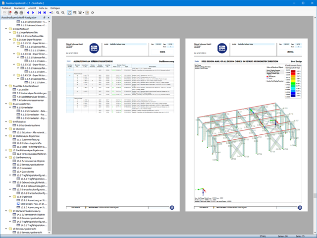
- Complete integration of the results into the RFEM/RSTAB printout report

- Realistic representation of interaction between a building and soil
- Realistic representation of the influences of the foundation components on each other
- Extensible library of soil properties
- Consideration of several soil samples (probes) at different locations, even outside the building
- Determination of settlements and stress diagrams as well as their graphical and tabular display

- Cross-section optimization
- Transfer of optimized sections to RFEM/RSTAB
- Design of any thin-walled section from RSECTION
- Representation of a stress diagram on a section
- Determination of normal, shear, and equivalent stresses
- Output of stress components for the individual member internal force types
- Detailed representation of stresses in all stress points
- Determination of the largest Δσ for each stress point (for example, for fatigue design)
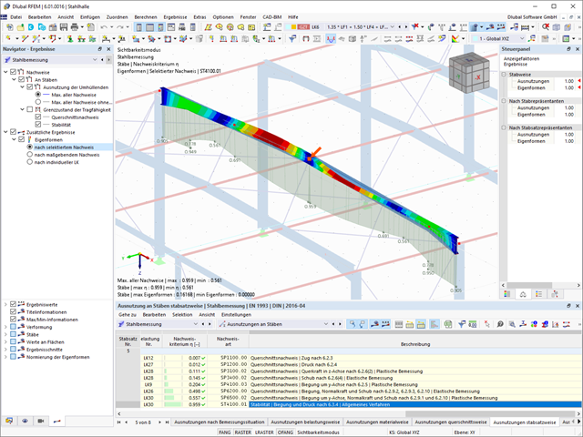
- Colored display of stresses and design ratios for a quick overview of the critical or oversized zones
- Output of parts lists

Did you know? The structural optimization in the programs RFEM and RSTAB is a completion of the parametric input. It is a parallel process beside the actual model calculation with all its regular calculation and design definitions. The add-on assumes that your model or block is built with a parametric context and is controlled in its entirety by global control parameters of the "optimization" type. Therefore, these control parameters have a lower and upper limit and a step size to delimit the optimization range. If you want to find optimal values for the control parameters, you have to specify an optimization criterion (for example, minimum weight) with the selection of an optimization method (for example, particle swarm optimization).
You can already find the cost and CO2 emission estimation in the material definitions. You can activate both options individually in each material definition. The estimation is based on a unit for unit cost or unit emission for members, surfaces, and solids. In this case, you can select whether to specify the units by weight, volume, or area.

For a response spectrum analysis of building models, you can display the sensitivity coefficients for the horizontal directions by story.
These key figures allow you to interpret the sensitivity to stability effects.

You have several options available to define masses for a modal analysis. While the masses due to self-weight are considered automatically, you can consider the loads and masses directly in a load case of the modal analysis type. Do you need more options? Select whether to consider full loads as masses, load components in the global Z-direction, or only the load components in the direction of gravity.
The program offers you an additional or alternative option for importing masses: A manual definition of load combinations as of which are the masses considered in the modal analysis. Have you selected a design standard? You can then create a design situation with the Seismic Mass combination type. Thus, the program automatically calculates a mass situation for the modal analysis according to the preferred design standard. In other words: The program creates a load combination on the basis of the preset combination coefficients for the selected standard. This contains the masses used for the modal analysis.

- Artificial intelligence technology (AI): Particle swarm optimization (PSO)
- Structure optimization according to the minimum weight or deformation
- Use of any number of optimization parameters
- Specification of variable ranges
- Optimization of cross-sections and materials
- Parameter definition types
- Optimization | Ascending or Optimization | Descending
- Application of parametric models and blocks
- Code-based JavaScript parametrization of blocks
- Optimization taking into account the design results
- Tabular display of the best model mutations
- Real-time display of the model mutations in the optimization process
- Model cost estimation by specifying unit prices
- Determination of the global warming potential GWP when realizing the model by estimating the CO2 equivalent
- Specification of weight-, volume-, and area-based units (price and CO2e)

In RFEM, you can use these three powerful eigenvalue solvers:
- Root of Characteristic Polynomial
- Method by Lanczos
- Subspace Iteration
RSTAB, on the other hand, provides you with these two eigenvalue solvers:
- Subspace Iteration
- Shifted inverse power method
The selection of the eigenvalue solver depends primarily on your model size.
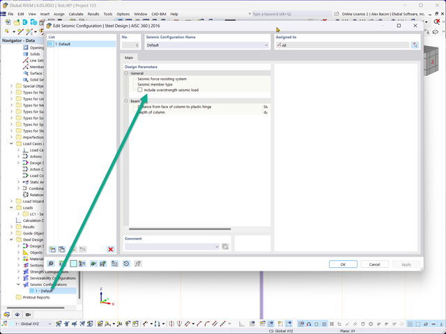
In the Concrete Design provides an option to perform seismic design according to AISC 341-16 for steel members.
Five SFRS types (Seismic Force-Resisting Systems) are available for this.
More Information
There are two methods that you can use for the optimization process, with which you can find optimal parameter values according to a weight or deformation criterion.
The most efficient method with the littlest calculation time is the near-natural particle swarm optimization (PSO). Have you heard or read about it? This artificial intelligence (AI) technology has a strong analogy to the behavior of flocks of animals, looking for a resting place. In such swarms, you can find many individuals (cf. optimization solution - for example, weight) who like to stay in a group and follow the group movement. Let's assume that each individual swarm member has a need to rest at an optimal resting place (cf. best solution - for example, lowest weight). This need increases as the resting place is approached. Thus, the swarm behavior is also influenced by the properties of the space (cf. result diagram).
Why the excursion into biology? Quite simply – the PSO process in RFEM or RSTAB proceeds in a similar way. The calculation run starts with an optimization result from a random assignment of the parameters to be optimized. It repeatedly determines new optimization results with varied parameter values, which are based on the experience of the previously performed model mutations. The process continues until the specified number of possible model mutations is reached.
As an alternative to this method, the program also offers you a batch processing method. This method attempts to check all possible model mutations by randomly specifying the values for the optimization parameters until a predetermined number of possible model mutations is reached.
After calculating a model mutation, both variants also check the respective activated design results of the add-ons. Furthermore, they save the variant with the corresponding optimization result and value assignment of the optimization parameters if the utilization is < 1.
You can determine the estimated total costs and emission from the respective sums of the individual materials. The sums of the materials are composed of the weight-based, volume-based, and area-based partial sums of the member, surface, and solid elements.
You enter the structural system and calculate the internal forces in the programs RFEM and RSTAB. You have full access to the extensive material and cross-section libraries. Did you know? You can also use the RSECTION program to create general cross-sections.
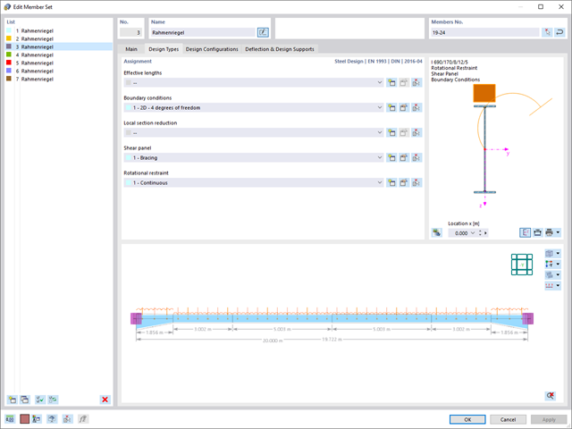
You find Steel Design fully integrated in the main programs. They automatically take into account the structure and the available calculation results. You can assign further entries for the aluminum design, such as effective lengths, cross-section reductions, or design parameters, to the objects to be designed. At many places of the program, you can easily select the elements graphically using the [Select] function.

Enter and model a soil solid directly in RFEM. You can combine the soil material models with all common RFEM add-ons.
This allows you to easily analyze the entire models with a complete representation of the soil-structure interaction.
All parameters required for the calculation are automatically determined from the material data that you have entered. The program then generates the stress-strain curves for each FE element.