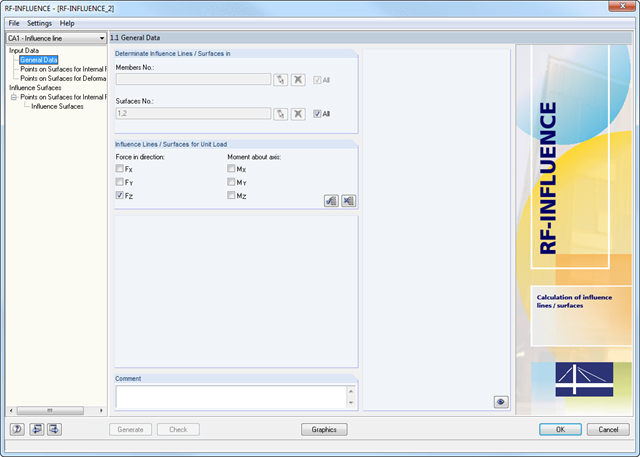
Member and surface models created in RFEM are analyzed at a particular point by applying a unit load with the previously defined load magnitude and direction. The module determines the way the unit load affects the internal forces at the inspected point.
This simulation is represented graphically by an influence line or influence surface resulting from the load magnitude of the force or moment at the inspected model point. The graphical representation can be used for further analyses or to check the behavior of the model.
The RF-INFLUENCE add-on module determines the influence lines and surfaces of models containing beams and surfaces.
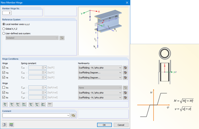
The member hinge nonlinearities "Scaffolding - N phiy / phiz" and "Scaffolding Diagram" enable the mechanical simulation of a tube joint with an inner stub between two member elements.
The equivalent model transfers the bending moment via the overpressed outer pipe and after positive locking additionally via the inner stub, depending on the compression state at the member end.
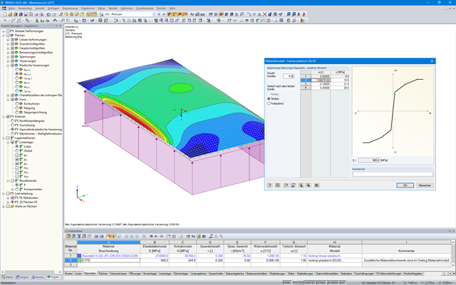
In RFEM, there is an option to couple surfaces with the stiffness types "Membrane" and "Membrane Orthotropic" with the material models "Isotropic Nonlinear Elastic 2D/3D" and "Isotropic Plastic 2D/3D" (add-on module RF-MAT NL is required).
This functionality enables simulation of the nonlinear strain behavior of ETFE foils, for example.

- 3D incompressible wind flow analysis with OpenFOAM® software package
- Direct model import from RFEM or RSTAB including neighboring and terrain models (3DS, IFC, STEP files)
- Model design via STL or VTP files independent of RFEM or RSTAB
- Simple model changes using Drag and Drop and graphical adjustment assistance
- Automatic corrections of the model topology with shrink wrap networks
- Option to add objects from the environment (buildings, terrain ...)
- Wind load determined over the height of the building, depending on standard-specific parameters (velocity, turbulence intensity)
- K-epsilon and K-omega turbulence models
- Automatic mesh generation adjusted to the selected depth of detail
- Parallel calculation with optimal utilization of the capacity of multicore computers
- Results in just minutes for low-resolution simulations (up to 1 million cells)
- Results within a few hours for simulations with medium/high resolution (1‑10 million cells)
- Graphical display of results on the Clipper/Slicer planes (scalar and vector fields)
- Graphical display of streamlines
- Streamline animation (optional video creation)
- Definition of point and line probes
- Display of aerodynamic pressure coefficients
- Graphical display of turbulence properties in the wind field
- Optional meshing using the boundary layer option for the area near the model surface
- Consideration of rough model surfaces possible
- Optional use of a seond-order numerical Order
- Multilingual user interface (for example, German, English, Spanish, French)
- Documentation possible in the RFEM and RSTAB printout report
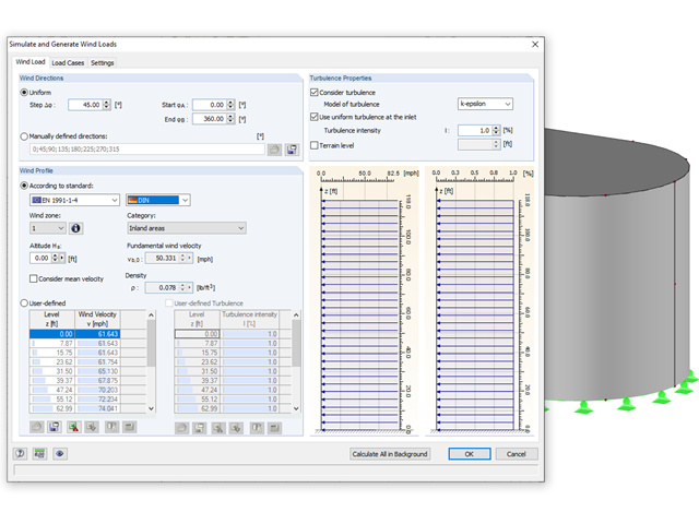
Rely on the Dlubal programs even in windy matters. RFEM and RSTAB provide a special interface for exporting models (that is, structures defined by members and surfaces) to RWIND 2. There, the wind directions to be analyzed for your project are defined by means of related angular positions about the vertical model axis. Furthermore, the elevation-dependent wind profile and turbulence intensity profile are defined on the basis of a wind standard. These specifications result in specific load cases, depending on the angle. For this, the fluid parameters, turbulence model properties, and iteration parameters that are all stored globally are helpful. You can extend these load cases by partial editing in the RWIND 2 environment using terrain or environment models from STL vector graphics.
As an alternative, you can also run RWIND 2 manually and without the interface application in RFEM or RSTAB. In this case, the structures and terrain environment in the program are directly modeled by imported STL and VTP files. You can define the height-dependent wind load and other fluid-mechanical data directly in RWIND 2.
Due to its versatile applicability, RWIND 2 is always at your side to support you in your individual projects.
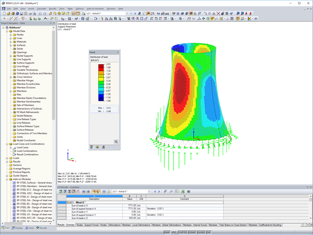
Work on your models with efficient and precise calculations in the digital wind tunnel. RWIND 2 uses a numerical CFD model (Computational Fluid Dynamics) to simulate wind flows around objects. Specific wind loads are generated from the simulation process for RFEM or RSTAB.
RWIND 2 performs this simulation using a 3D volume mesh. The program provides automatic meshing; you can easily set the entire mesh density as well as the local mesh refinement on the model using a few parameters. A numerical solver for incompressible turbulent flows is used to calculate the wind flows and the surface pressures on the model. The results are then extrapolated to your model. RWIND 2 is designed to work with different numerical solvers.
We currently recommend using the OpenFOAM® software package, which has provided very good results in our tests and is also a frequently used tool for CFD simulations. Alternative numerical solvers are under development.
Always keep an eye on your results. In addition to the resulting load cases in RFEM or RSTAB (see below), the results from the aerodynamics analysis in RWIND 2 represent the flow problem as a whole:
- Pressure on structure surface
- Pressure field about structure geometry
- Velocity field about structure geometry
- Velocity vectors about structure geometry
- Flow lines about structure geometry
- Forces on member-shaped structures that were originally generated from member elements
- Convergence diagram
- Direction and size of the flow resistance of the defined structures
These results are displayed in the RWIND 2 environment and evaluated graphically. The flow results around the structure geometry in the overall display are rather confusing, but the program has a solution for this. In order to present clearly arranged results, freely movable section planes are displayed for the separate display of the 'solid results' in a plane. Accordingly, for the 3D branched streamline result, the program presents you an animated display in the form of moving lines or particles in addition to the static one. This option helps to represent the wind flow as a dynamic effect.
You can export all results as a picture or, especially for the animated results, as a video.
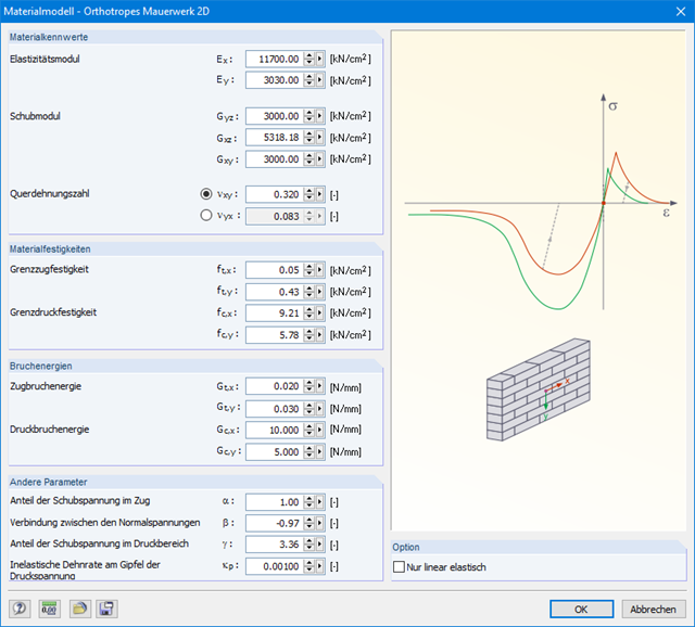
The material model Orthotropic Masonry 2D is an elastoplastic model that additionally allows softening of the material, which can be different in the local x- and y-directions of a surface. The material model is suitable for (unreinforced) masonry walls with in-plane loads.
.png?mw=640&hash=9a883491884955dbc811b6573882f2d9b2702a99)
The RWIND Simulation program for generating wind loads based on CFD can be utilized in different languages; for example, in:
- German
- English
- Czech
- Spanish
- French
- Italian
- Polish
- Portuguese
- Russian
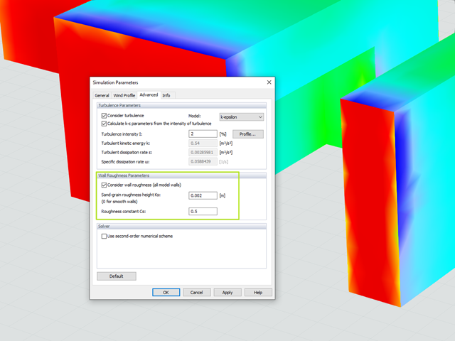
Utilize the RWIND Simulation program to consider a surface roughness of the model surface by applying a modified wall boundary condition. The numerical model is based on the assumption that grains with a certain diameter are arranged homogeneously on the model surface, similar to sandpaper. The grain diameter is described with the parameter Ks and the distribution with the parameter Cs. By considering the wall roughness, the numerical flow simulation can capture reality more closely.
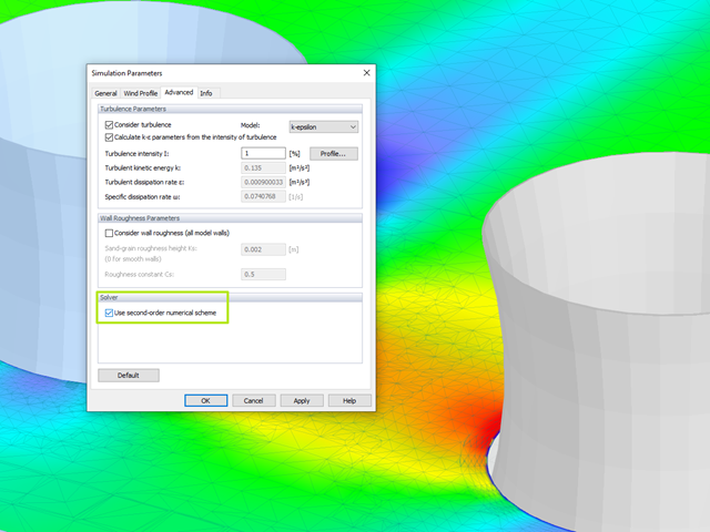
The volume space in RWIND Simulation can optionally be discretized with the second-order theory between the cells.
This extended approach usually results in more accurate results despite poorer convergence behavior.
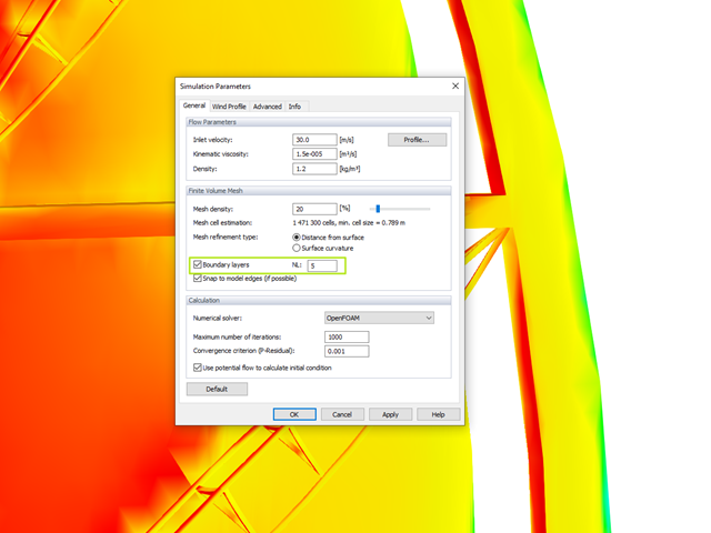
The meshing algorithm of RWIND Simulation uses the boundary layer option to mesh the area near the model surface with a voluminous layer mesh. The number of layers is controlled by a user-defined parameter.
This fine mesh in the area of the model surface helps to represent the wind velocity close to the surface.
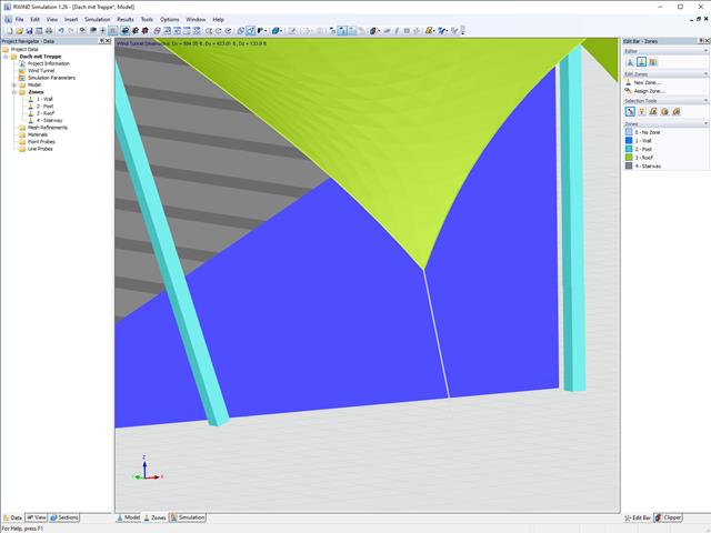
In RWIND Simulation, it is possible to divide the model in different zones. This allows for different surface roughness to be assigned to the zones. In addition, local results can be better evaluated.

Compared to the RF-FORM-FINDING add-on module (RFEM 5), the following new features have been added to the Form-Finding add-on for RFEM 6:
- Specification of all form-finding load boundary conditions in one load case
- Storage of form-finding results as initial state for further model analysis
- Automatic assignment of the form-finding initial state via combination wizards to all load situations of a design situation
- Additional form-finding geometry boundary conditions for members (unstressed length, maximum vertical sag, low-point vertical sag)
- Additional form-finding load boundary conditions for members (maximum force in member, minimum force in member, horizontal tension component, tension at i-end, tension at j-end, minimum tension at i-end, minimum tension at j-end)
- Material types "Fabric" and "Foil" in material library
- Parallel form-findings in one model
- Simulation of sequentially building form-finding states in connection with the Construction Stages Analysis (CSA) add-on

Compared to the RF‑SOILIN add-on module (RFEM‑5), the following new features have been added to the Geotechnical Analysis add-on for RFEM 6:
- Creation of the layered soil as a 3D model from the entirety of the defined soil samples
- Recognized material law according to Mohr-Coulomb for soil simulation
- Graphical and tabular output of stresses and strains at any depth of the soil
- Optimal consideration of the soil-structure interaction on the basis of an overall model

If you are looking for models to practice on or as inspiration for your projects, you've come to the right place. We offer a vast number of structural analysis models to download, such as RFEM, RSTAB, or RWIND files.
Models to Download
- Calculation of stationary incompressible turbulent wind flow using the SimpleFOAM solver from the OpenFOAM® software package
- Numerical scheme according to the first and second order
- Turbulence models RAS k-ω and RAS k-ε
- Consideration of surface roughness depending on model zones
- Model design via VTP, STL, OBJ, and IFC files
- Operation via bidirectional interface of RFEM or RSTAB for importing model geometries with standard-based wind loads and exporting wind load cases with probe-based printout report tables
- Intuitive model changes via drag & drop and graphical adjustment assistance
- Generation of a shrink-wrap mesh envelope around the model geometry
- Consideration of environmental objects (buildings, terrain, and so on)
- Height-dependent description of the wind load (wind speed and turbulence intensity)
- Automatic meshing depending on a selected depth of detail
- Consideration of layer meshes near the model surfaces
- Parallelized calculation with optimal utilization of all processor cores of a computer
- Graphical output of the surface results on the model surfaces (surface pressure, Cp coefficients)
- Graphical output of the flow field and vector results (pressure field, velocity field, turbulence – k-ω field, and turbulence – k-ε field, velocity vectors) on Clipper/Slicer planes
- Display of 3D wind flow via animated streamline graphics
- Definition of point and line probes
- Multilingual user interface (German, English, Czech, Spanish, French, Italian, Polish, Portuguese, Russian, and Chinese)
- Calculations of several models in one batch process
- Generator for creating rotated models to simulate different wind directions
- Optional interruption and continuation of the calculation
- Individual color panel per result graphic
- Display of diagrams with separate output of results on both sides of a surface
- Output of the dimensionless wall distance y+ in the mesh inspector details for the simplified model mesh
- Determination of the shear stress on the model surface from the flow around the model
- Calculation with an alternative convergence criterion (you can select between the residual types pressure or flow resistance in the simulation parameters)
- Calculation of transient incompressible turbulent wind flow with the BlueDyMSolver solver
- LES SpalartAllmarasDDES turbulence model
- Consideration of stationary solution as initial state for transient calculation
- Automatic determination of analysis period and time steps
- Use of intermediate results during the calculation
- Organized display of time-varying results via time step units
- Diagram of drag force and point probe results over analysis time
- Display of line probe results for any time steps in a diagram
- Freely adjustable wind permeability for surfaces (Go to Product Feature)
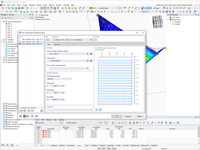
To model structures in RWIND Basic, you find a special application in RFEM and RSTAB. Here, you define the wind directions to be analyzed by means of related angular positions about the vertical model axis. At the same time, you define the elevation-dependent wind profile on the basis of a wind standard. In addition to these specifications, you can use the stored calculation parameters to determine your own load cases for a stationary calculation per each angular position.
As an alternative, you can also use the RWIND Basic program manually, without the interface application in RFEM or RSTAB. In this case, RWIND Basic models the structures and terrain environment directly from the imported VTP, STL, OBJ, and IFC files. You can define the height-dependent wind load and other fluid-mechanical data directly in RWIND Basic.