
Did you know that you can also display the moment-axial force interaction diagrams (M‑N diagrams) graphically? This allows you to display the cross-section resistance in the case of an interaction of a bending moment and an axial force. In addition to the interaction diagrams related to the cross-section axes (My‑N diagram and Mz‑N diagram), you can also generate an individual moment vector to create an Mres‑N interaction diagram. You can display the section plane of the M‑N diagrams in the 3D interaction diagram. The program displays the corresponding value pairs of the ultimate limit state in a table. The table is dynamically linked to the diagram so that the selected limit point is also displayed in the diagram.
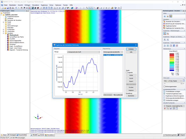
Always keep an eye on your results. In addition to the resulting load cases in RFEM or RSTAB (see below), the results from the aerodynamics analysis in RWIND 2 represent the flow problem as a whole:
- Pressure on structure surface
- Pressure field about structure geometry
- Velocity field about structure geometry
- Velocity vectors about structure geometry
- Flow lines about structure geometry
- Forces on member-shaped structures that were originally generated from member elements
- Convergence diagram
- Direction and size of the flow resistance of the defined structures
These results are displayed in the RWIND 2 environment and evaluated graphically. The flow results around the structure geometry in the overall display are rather confusing, but the program has a solution for this. In order to present clearly arranged results, freely movable section planes are displayed for the separate display of the 'solid results' in a plane. Accordingly, for the 3D branched streamline result, the program presents you an animated display in the form of moving lines or particles in addition to the static one. This option helps to represent the wind flow as a dynamic effect.
You can export all results as a picture or, especially for the animated results, as a video.

- Calculation of stationary incompressible turbulent wind flow using the SimpleFOAM solver from the OpenFOAM® software package
- Numerical scheme according to the first and second order
- Turbulence models RAS k-ω and RAS k-ε
- Consideration of surface roughness depending on model zones
- Model design via VTP, STL, OBJ, and IFC files
- Operation via bidirectional interface of RFEM or RSTAB for importing model geometries with standard-based wind loads and exporting wind load cases with probe-based printout report tables
- Intuitive model changes via drag & drop and graphical adjustment assistance
- Generation of a shrink-wrap mesh envelope around the model geometry
- Consideration of environmental objects (buildings, terrain, and so on)
- Height-dependent description of the wind load (wind speed and turbulence intensity)
- Automatic meshing depending on a selected depth of detail
- Consideration of layer meshes near the model surfaces
- Parallelized calculation with optimal utilization of all processor cores of a computer
- Graphical output of the surface results on the model surfaces (surface pressure, Cp coefficients)
- Graphical output of the flow field and vector results (pressure field, velocity field, turbulence – k-ω field, and turbulence – k-ε field, velocity vectors) on Clipper/Slicer planes
- Display of 3D wind flow via animated streamline graphics
- Definition of point and line probes
- Multilingual user interface (German, English, Czech, Spanish, French, Italian, Polish, Portuguese, Russian, and Chinese)
- Calculations of several models in one batch process
- Generator for creating rotated models to simulate different wind directions
- Optional interruption and continuation of the calculation
- Individual color panel per result graphic
- Display of diagrams with separate output of results on both sides of a surface
- Output of the dimensionless wall distance y+ in the mesh inspector details for the simplified model mesh
- Determination of the shear stress on the model surface from the flow around the model
- Calculation with an alternative convergence criterion (you can select between the residual types pressure or flow resistance in the simulation parameters)

As you've already learned, the results of a Modal Analysis load case are displayed in the program after a successful calculation. You can thus immediately see the first mode shape graphically or as an animation. You can also easily adjust the representation of the mode shape standardization. Do that directly in the Results navigator, where you have one of four options for the visualization of the mode shapes available for the selection:
- Scaling the value of the mode shape vector uj to 1 (considers the translation components only)
- Selecting the maximum translational component of the eigenvector and setting it to 1
- Considering the entire eigenvector (including the rotation components), selecting the maximum, and setting it to 1
- Setting the modal mass mi for each mode shape to 1 kg
You can find a detailed explanation of the mode shape standardization in the OnlineManual here.
.png?mw=640&hash=5a991f211d984ac624978f514e70c53da263e5d9)
Depending on the axial force N, you can generate a moment curvature line for any moment vector. The program also shows you the value pairs of the displayed diagram in a table. Furthermore, you can activate the secant stiffness and tangent stiffness of the reinforced concrete cross-section, belonging to the moment curvature diagram, as an additional diagram.
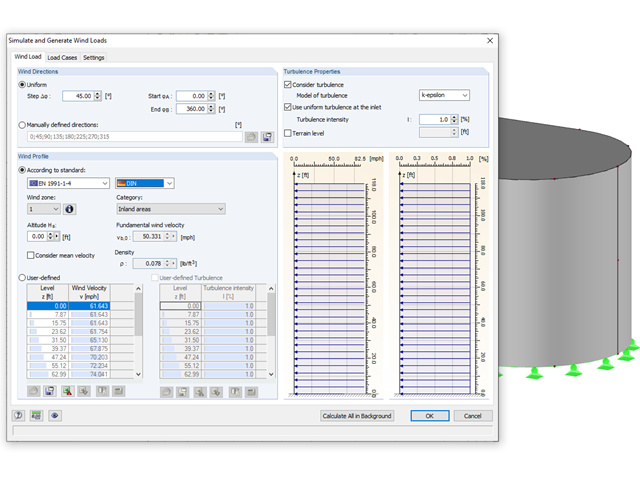
Rely on the Dlubal programs even in windy matters. RFEM and RSTAB provide a special interface for exporting models (that is, structures defined by members and surfaces) to RWIND 2. There, the wind directions to be analyzed for your project are defined by means of related angular positions about the vertical model axis. Furthermore, the elevation-dependent wind profile and turbulence intensity profile are defined on the basis of a wind standard. These specifications result in specific load cases, depending on the angle. For this, the fluid parameters, turbulence model properties, and iteration parameters that are all stored globally are helpful. You can extend these load cases by partial editing in the RWIND 2 environment using terrain or environment models from STL vector graphics.
As an alternative, you can also run RWIND 2 manually and without the interface application in RFEM or RSTAB. In this case, the structures and terrain environment in the program are directly modeled by imported STL and VTP files. You can define the height-dependent wind load and other fluid-mechanical data directly in RWIND 2.
Due to its versatile applicability, RWIND 2 is always at your side to support you in your individual projects.
- 3D incompressible wind flow analysis with OpenFOAM® software package
- Direct model import from RFEM or RSTAB including neighboring and terrain models (3DS, IFC, STEP files)
- Model design via STL or VTP files independent of RFEM or RSTAB
- Simple model changes using Drag and Drop and graphical adjustment assistance
- Automatic corrections of the model topology with shrink wrap networks
- Option to add objects from the environment (buildings, terrain ...)
- Wind load determined over the height of the building, depending on standard-specific parameters (velocity, turbulence intensity)
- K-epsilon and K-omega turbulence models
- Automatic mesh generation adjusted to the selected depth of detail
- Parallel calculation with optimal utilization of the capacity of multicore computers
- Results in just minutes for low-resolution simulations (up to 1 million cells)
- Results within a few hours for simulations with medium/high resolution (1‑10 million cells)
- Graphical display of results on the Clipper/Slicer planes (scalar and vector fields)
- Graphical display of streamlines
- Streamline animation (optional video creation)
- Definition of point and line probes
- Display of aerodynamic pressure coefficients
- Graphical display of turbulence properties in the wind field
- Optional meshing using the boundary layer option for the area near the model surface
- Consideration of rough model surfaces possible
- Optional use of a seond-order numerical Order
- Multilingual user interface (for example, German, English, Spanish, French)
- Documentation possible in the RFEM and RSTAB printout report
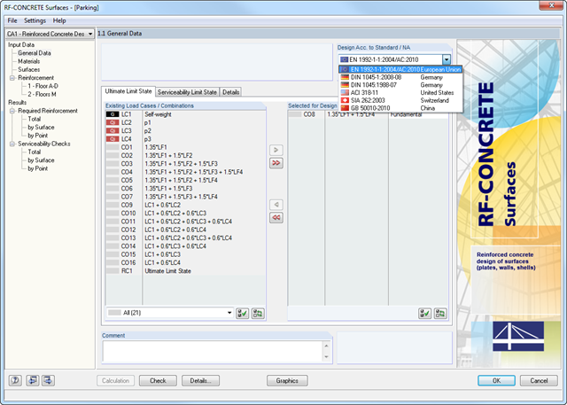
- Free definition of two or three reinforcement layers in the ultimate limit state
- Vectorial representation of the main stress directions of internal forces allowing optimal orientation adjustment of the third reinforcement layer to the actions
- Design alternatives to avoid compression or shear reinforcement
- Design of surfaces as deep beams (theory of membranes)
- Option to define basic reinforcements for top and bottom reinforcement layers
- Definition of designed reinforcement for serviceability limit state design
- Result output in points of any selected grid
- Optional extension of the module with nonlinear deformation analysis. The calculation is performed in RF‑CONCRETE Deflect by reducing the stiffness according to the standard, or in RF‑CONCRETE NL by the general nonlinear calculation determining the stiffness reduction in an iterative process.
- Design with design moments at column edges
- Precise breakdown of reasons for failed design
- Design details of all design locations for better traceability of reinforcement determination
- Export of isolines for the longitudinal reinforcement in a DXF file for further use in CAD programs as a basis for reinforcement drawings
Comprehensive and easy options in the individual input windows facilitate the representation of the structural system:
Nodal Supports
- The support type of each node is editable.
- It is possible to define a warp stiffening on each node. The resulting warp spring is determined automatically using the input parameters.
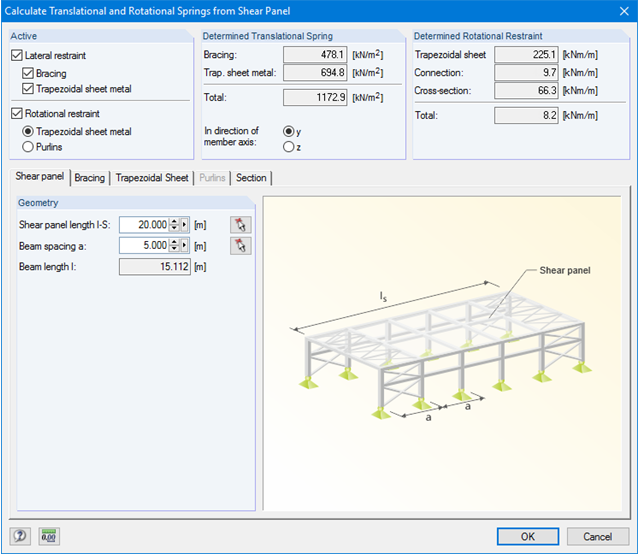
Elastic member foundation
- In the case of elastic member foundations, you can manually enter spring constants.
- Alternatively, you can use the various options to define the rotational and translational springs from a shear panel.
Member End Springs
- RF-/FE-LTB calculates the individual spring constants automatically. You can use the dialog boxes and detailed pictures to represent a translational spring by connecting component, a rotational spring by a connecting column, or a warping stiffener (available types: end plate, channel section, angle, connecting column, cantilevered portion).
Member Hinges
- If there are no member hinges defined in RFEM/RSTAB for the set of members, you can define them directly in the RF-/FE-LTB add-on module.
Load Data
- The nodal and member loads of the selected load cases and combinations are displayed in separate windows. There you can edit, delete, or add them individually.
Imperfections
- RF-/FE-LTB automatically applies the imperfections by scaling the lowest eigenvector.

Do you know exactly how the form-finding is performed? First, the form-finding process of the load cases with the load case category "Prestress" shifts the initial mesh geometry to an optimally balanced position by means of iterative calculation loops. For this task, the program uses the Updated Reference Strategy (URS) method by Prof. Bletzinger and Prof. Ramm. This technology is characterized by equilibrium shapes that, after the calculation, comply almost exactly with the initially specified form-finding boundary conditions (sag, force, and prestress).
In addition to the pure description of the expected forces or sags on the elements to be formed, the integral approach of the URS also enables a consideration of regular forces. In the overall process, this allows, for example, for a description of the self-weight or a pneumatic pressure by means of corresponding element loads.
All these options give the calculation kernel the potential to calculate anticlastic and synclastic forms that are in an equilibrium of forces for planar or rotationally symmetric geometries. In order to be able to realistically implement both types individually or together in one environment, the calculation provide you with two ways to describe the form-finding force vectors:
- Tension method - description of the form-finding force vectors in space for planar geometries
- Projection method - description of the form-finding force vectors on a projection plane with fixation of the horizontal position for conical geometries
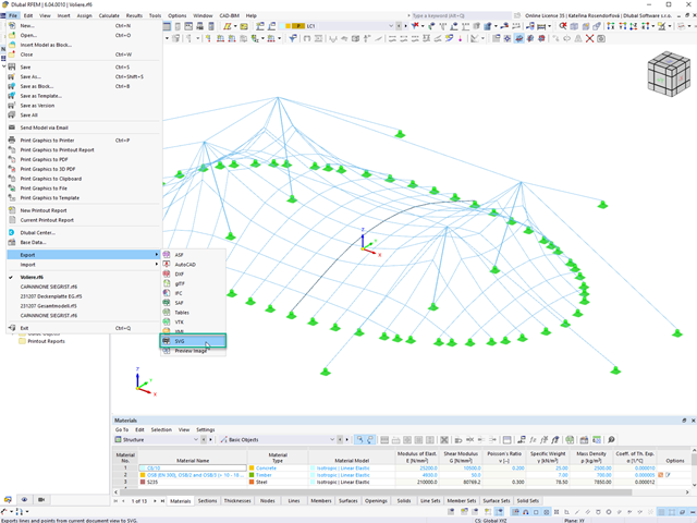
In RFEM 6 and RSTAB 9, you can export line graphics to the SVG format (vector graphics).
SVG stands for Scalable Vector Graphics and is an XML-based file format for displaying two-dimensional vector graphics. These vector graphics can be scaled without loss. It is possible to edit the SVG files using text editors, embed them on websites, and open them in the usual browsers.
By solving the numerical flow problem, you can obtain the following results on and around the model:
- Pressure on structure surface
- Coefficient Cp distribution on the structure surfaces
- Pressure field about the structure geometry
- Velocity field about the structure geometry
- Turbulence k-ω field about the structure geometry
- Turbulence k-ε field about the structure geometry
- Velocity vectors about the structure geometry
- Streamlines about the structure geometry
- Forces on member-shaped structures that were originally generated from member elements
- Convergence diagram
- Direction and size of the flow resistance of the defined structures
Despite this amount of information, RWIND 2 remains clearly arranged, as is typical for the Dlubal programs. You can specify freely definable zones for a graphic evaluation. Voluminously displayed flow results about the structure geometry are often confusing – you know the problem for sure. That's why RWIND Basic provides freely movable section planes for the separate display of the "solid results" in a plane. For the 3D branched streamline result, you have an option to select between a static and an animated display in the form of moving line segments or particles. This option helps you to represent the wind flow as a dynamic effect.
You can export all results as a picture or, especially for the animated results, as a video.