
You can neglect openings with a certain area in the building model calculation. This function can be activated in the global settings of the building stories. A warning message appears saying that the openings have been neglected.
.png?mw=640&hash=9de889f94dda719e52d438f3fb6a495d2dce9a98)
Use the "Independent mesh preferred" option in the FE mesh settings to create an independent FE mesh for the integrated objects.
This allows you to generate a significantly more detailed and precise FE mesh for individual objects that are integrated into one another.
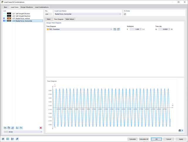
It is necessary to enter the required force-time diagrams. They can be combined in load cases or load combinations of the type Time History Analysis | Time Diagrams with the loading in order to define where and in which direction the force-time diagrams act.
The second option is to enter acceleration-time diagrams, which can be used in the load cases of the Time History Analysis | Accelerogram type.
All calculation parameters are specified in the time history analysis settings. These include, for example, the type of analysis method and the maximum calculation time.
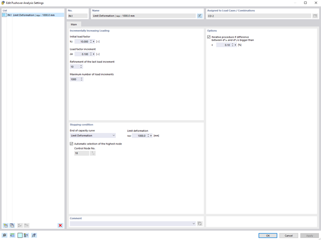
The pushover analysis is managed by a newly introduced analysis type in the load combinations. Here, you have access to the selection of the horizontal load distribution and direction, the selection of a constant load, the selection of the desired response spectrum for the determination of the target displacement, and the pushover analysis settings tailored to the pushover analysis.
In the pushover analysis settings, you can modify the increment of the increasing horizontal load and specify the stopping condition for the analysis. Furthermore, it is possible to easily adjust the precision for the iterative determination of the target displacement.
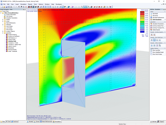
Use RWIND 2 Pro to easily apply a permeability to a surface. All you need is the definition of
- the Darcy coefficient D,
- the inertial coefficient I, and
- the length of the porous medium in the direction of flow L,
to define a pressure boundary condition between the front and back of a porous zone. Due to this setting, you obtain the flow through this zone with a two-part result display on both sides of the zone area.
But that's not all. Furthermore, the generation of a simplified model recognizes permeable zones and takes into account the corresponding openings in the model coating. Can you waive an elaborate geometric modeling of the porous element? Understandable – we have good news for you then! With a pure definition of the permeability parameters, you can avoid complex geometric modeling of the porous element. Use this feature to simulate permeable scaffolding, dust curtains, mesh structures, and so on.
More Information
The soil solids that you want to analyze are summarized in soil massifs.
Use the soil samples as a basis for a definition of the respective soil massif. This way, the program allows for user-friendly generation of the massif, including the automatic determination of the layer interfaces from the sample data, as well as the groundwater level and the boundary surface supports.
Soil massifs provide you with the option to specify a target FE mesh size independently of the global setting for the rest of the structure. You can thus consider the various requirements of the building and soil in the entire model.
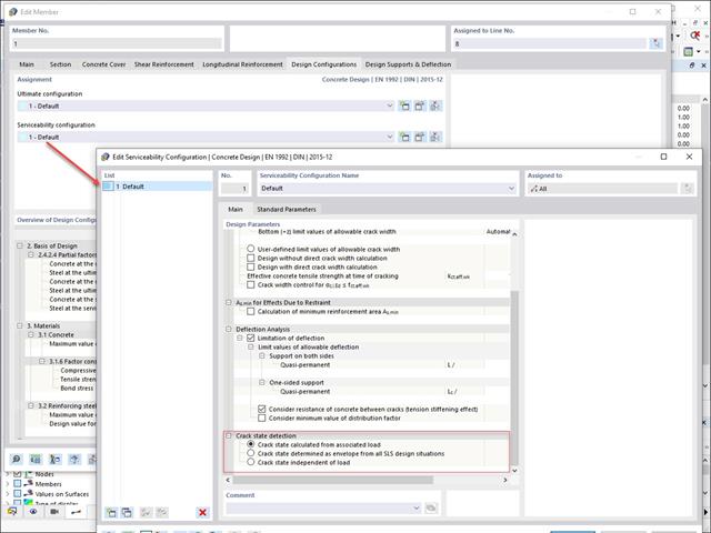
Various design parameters of the cross-sections can be adjusted in the serviceability limit state configuration. The applied cross-section condition for the deformation and crack width analysis can be controlled there.
For this, the following settings can be activated:
- Crack state calculated from associated load
- Crack state determined as an envelope from all SLS design situations
- Cracked state of cross-section - independent of load

Have you already discovered the tabular and graphical output of masses in mesh points? That's right, this is also part of the modal analysis results in RFEM 6. This way, you can check the imported masses that depend on various settings of the modal analysis. They can be displayed in the Masses in Mesh Points tab of the Results table. The table provides you with an overview of the following results: Mass - Translational Direction (mX, mY, mZ), Mass - Rotational Direction (mφX, mφY, mφZ), and the Sum of Masses. Would it be best for you to have a graphical evaluation as quickly as possible? Then you can also graphically display the masses in mesh points.

As you've already learned, the results of a Modal Analysis load case are displayed in the program after a successful calculation. You can thus immediately see the first mode shape graphically or as an animation. You can also easily adjust the representation of the mode shape standardization. Do that directly in the Results navigator, where you have one of four options for the visualization of the mode shapes available for the selection:
- Scaling the value of the mode shape vector uj to 1 (considers the translation components only)
- Selecting the maximum translational component of the eigenvector and setting it to 1
- Considering the entire eigenvector (including the rotation components), selecting the maximum, and setting it to 1
- Setting the modal mass mi for each mode shape to 1 kg
You can find a detailed explanation of the mode shape standardization in the OnlineManual here.
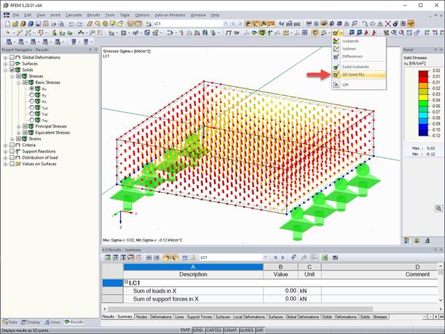
The results of solid stresses can be displayed as colored 3D points in the finite elements.

When defining the input data for the modal analysis load case, you can consider a load case whose stiffnesses represent the initial position for the modal analysis. How do you do that? As shown in the image, select the "Consider initial state from" option. Now, open the "Initial State Settings" dialog box and define the type Stiffness as the initial state. In this load case, as of which is the initial state taken into account, you can consider the stiffness of the structural system when the tension members fail. The purpose of all of this: The stiffness from this load case is considered in the modal analysis. Thus, you obtain a clearly flexible system.

- A wide range of cross-sections, such as rectangular sections, square sections, T‑sections, circular sections, built-up cross-sections, irregular parametric cross-sections, and many others (suitability for design depends on the selected standard)
- Design of cross-laminated timber (CLT)
- Design of timber-based materials and laminated veneer lumber according to EC 5
- Design of tapered and curved members (design method according to the standard)
- Adjustment of the essential design factors and standard parameters is possible
- Flexibility due to detailed setting options for basis and extent of calculations
- Fast and clear results output for an immediate overview of the result distribution after the design
- Detailed output of the design results and essential formulas (comprehensible and verifiable result path)
- Numerical results clearly arranged in tables and graphical display of the results in the model
- Integration of the output into the RFEM/RSTAB printout report
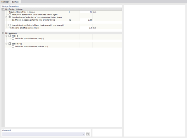
RFEM/RSTAB also provides a range of functions for the case of a fire. The program allows for the automatic generation of load and result combinations for the accidental design situation of fire design. The members to be designed with the corresponding internal forces are imported directly from RFEM/RSTAB. Also, all information about the material and cross-section is stored. You don't need to do anything else.
You only define the parameters relevant for the fire resistance design by assigning a fire resistance configuration to the members and surfaces to be designed. Moreover, you can also make further detailed settings, such as the definition of the fire exposure on one side up to all sides.
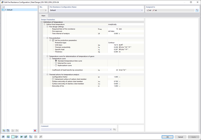
The structural analysis programs RFEM/RSTAB offer you a wide range of automated functions that make your dayily work easier. One of them is the automatic generation of load and result combinations for the accidental design situation of fire design. The members to be designed with the corresponding internal forces are imported directly from RFEM/RSTAB. You don't need to do anything else. The program has also already stored all information about the material and cross-section for you.
By assigning a fire resistance configuration to the members to be designed, you define the parameters relevant for the fire resistance design. Here you can manually specify the critical steel temperature at the design time. Or let the program to determine the temperature determined automatically for a specified fire duration. You can select from various fire temperature curves and fire protection measures. It is also possible to make further detailed settings, such as the definition of the fire exposure on all sides or three sides
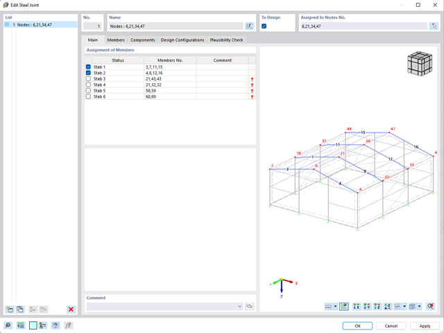
- For a new connection model, you have to select a node in the RFEM model
- After selecting a node, the members connected to the node are automatically recognized and assigned
- In the window for assigning members, select the ones that will be assigned to the connection
- The members marked by us are displayed in the preview window on the right
- Connections can be modeled for multiple nodes in a structure.
- For member settings, select the ones to be supported
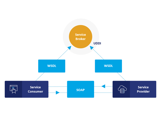
Communication is the key to success. This also applies to a client-server relation. WebService and API provides you with an XML based information exchange system for direct client-server communication. Programs, objects, messages, or documents can be integrated into these systems. For example, a web service protocol of the HTTP type runs for the client-server communication when you are looking for something in the Internet using a search engine.
Now back to Dlubal Software. In our case, the client is your programming environment (.NET, Python, JavaScript) and the service provider is RFEM 6. Client-server communication allows you to send requests to and receive feedback from RFEM, RSTAB, or RSECTION.
What is the difference between WebService and an API?
- WebService is a collection of open source protocols and standards used to exchange data between systems and applications. In contrast, an application programming interface (API), is a software interface through which two applications can interact without a user being involved.
- Thus, all web services are APIs, but not all APIs are web services.
What are the advantages of the WebService technology?
You can communicate more quickly within and between organizations.A service can be independent of other services.Webservice allows you to use your application to make your message or feature available to the rest of the world.Webservice helps you to exchange data between different applications and platforms Several applications can communicate, exchange data, and share services with each other. SOAP ensures that programs created on different platforms and based on different programming languages can exchange data securely.
Communication between the web service client and server is optionally encrypted via the https protocol. To do this, you can install an SSL certificate with the corresponding private key in the settings.
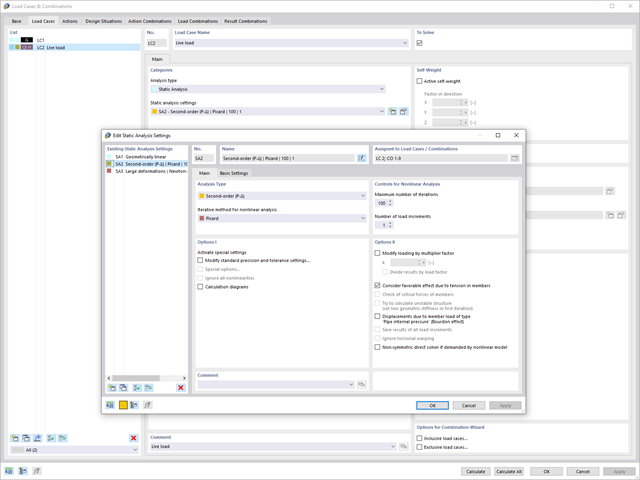
Use the new structural analysis setting to provide load cases and load combinations with individual global calculation parameters.
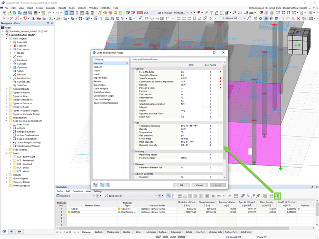
You can now change certain units in the form of a tabular user interface. You can now change certain units in the form of a tabular user interface.
- Calculation of stationary incompressible turbulent wind flow using the SimpleFOAM solver from the OpenFOAM® software package
- Numerical scheme according to the first and second order
- Turbulence models RAS k-ω and RAS k-ε
- Consideration of surface roughness depending on model zones
- Model design via VTP, STL, OBJ, and IFC files
- Operation via bidirectional interface of RFEM or RSTAB for importing model geometries with standard-based wind loads and exporting wind load cases with probe-based printout report tables
- Intuitive model changes via drag & drop and graphical adjustment assistance
- Generation of a shrink-wrap mesh envelope around the model geometry
- Consideration of environmental objects (buildings, terrain, and so on)
- Height-dependent description of the wind load (wind speed and turbulence intensity)
- Automatic meshing depending on a selected depth of detail
- Consideration of layer meshes near the model surfaces
- Parallelized calculation with optimal utilization of all processor cores of a computer
- Graphical output of the surface results on the model surfaces (surface pressure, Cp coefficients)
- Graphical output of the flow field and vector results (pressure field, velocity field, turbulence – k-ω field, and turbulence – k-ε field, velocity vectors) on Clipper/Slicer planes
- Display of 3D wind flow via animated streamline graphics
- Definition of point and line probes
- Multilingual user interface (German, English, Czech, Spanish, French, Italian, Polish, Portuguese, Russian, and Chinese)
- Calculations of several models in one batch process
- Generator for creating rotated models to simulate different wind directions
- Optional interruption and continuation of the calculation
- Individual color panel per result graphic
- Display of diagrams with separate output of results on both sides of a surface
- Output of the dimensionless wall distance y+ in the mesh inspector details for the simplified model mesh
- Determination of the shear stress on the model surface from the flow around the model
- Calculation with an alternative convergence criterion (you can select between the residual types pressure or flow resistance in the simulation parameters)
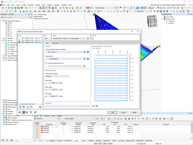
Discover the new features in RFEM and RSTAB for the determination of wind loads using RWIND:
- Useful load wizards for generating wind load cases with different flow fields in different wind directions
- Wind load cases with freely assignable analysis settings including a user-defined specification of the wind tunnel size and wind profile
- Comprehensive display of the wind tunnel with input wind profile and turbulence intensity profile
- Visualization and use of the RWIND simulation results
- Global definition of a terrain (horizontal planes, inclined plane, table)
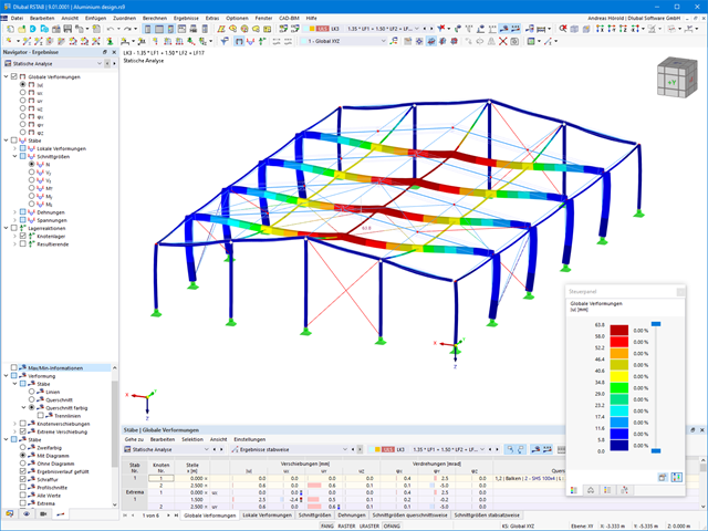
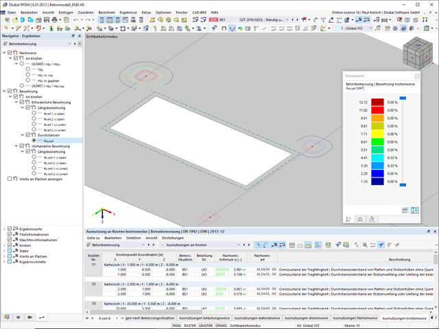
Also, on the rendered model, you see your results in a clear color display. This allows you to precisely recognize the deformation or internal forces of a member, for example. If you want to set the colors and value ranges, you can do so in the control panel.
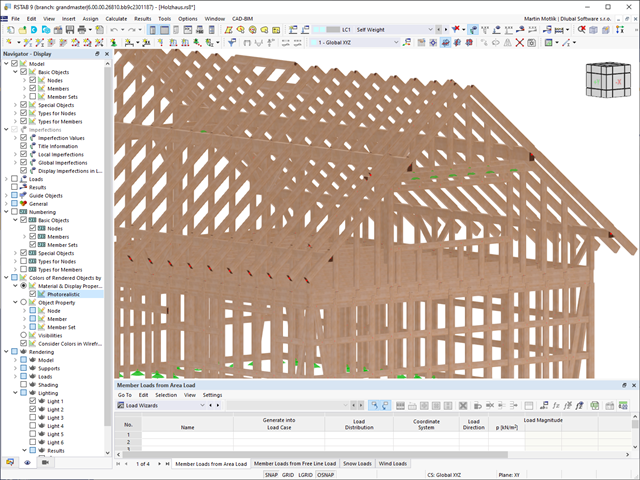
The model is rendered photorealistically (optionally with textures). This gives you the advantage that you always have immediate control of the input. You can freely adjust the display colors and save them separately for the screen as well as for the printout.
Go to Explanatory Video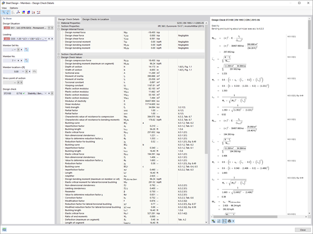
Compared to the RF‑/STEEL EC3 add-on module (RFEM 5 / RSTAB 8), the following new features have been added to the Steel Design add-on for RFEM 6 / RSTAB 9:
- In addition to Eurocode 3, other international standards are integrated (such as AISC 360, CSA S16, GB 50017, SP 16.13330)
- Consideration of hot-dip galvanizing (DASt guideline 027) in the fire protection design according to EN 1993‑1‑2
- Input option for transverse stiffeners that can be taken into account in the shear buckling analysis
- Lateral-torsional buckling can also be checked for hollow sections (for example, relevant for slender, high rectangular hollow sections)
- Automatic detection of members or member sets valid for the design (for example, automatic deactivation of members with invalid material or members already contained in a member set)
- Design settings can be adjusted individually for each member
- Graphical display of the results in the gross section or the effective section
- Output of the used design check formulas (including a reference to the used equation from the standard)

Compared to the RF‑/STEEL add-on module (RFEM 5 / RSTAB 8), the following new features have been added to the Stress-Strain Analysis add-on for RFEM 6 / RSTAB 9:
- Treatment of members, surfaces, solids, welds (line welded joints between two and three surfaces with subsequent stress design)
- Output of stresses, stress ratios, stress ranges, and strains
- Limit stress depending on the assigned material or a user-defined input
- Individual specification of the results to be calculated through freely assignable setting types
- Non-modal result details with prepared formula display and additional result display on the cross-section level of members
- Output of the design check formulas used

The Dlubal structural analysis software does a lot of work for you. The input parameters, which are relevant for the selected standards, are suggested by the program in accordance with the rules. Furthermore, you can enter response spectra manually.
Load cases of the type Response Spectrum Analysis define the direction in which response spectra act and which eigenvalues of the structure are relevant for the analysis. In the spectral analysis settings, you can define details for the combination rules, damping (if applicable), and zero-period acceleration (ZPA).

- Selection of nodes in the RFEM model, automatic recognition and assignment of the members connected to the node
- Many predefined components available for easy input of typical connection situations (for example, end plates, cleats, fin plates)
- Universally applicable basic components (plates, welds, auxiliary planes) for entering complex connection situations
- No manual editing of the FE model required by the user, the essential calculation settings can be changed via the configuration settings
- Automatic adaptation of the connection geometry, even if the members are subsequently edited, due to the relative relation of the components to each other
- Parallel to the input, a plausibility check is carried out by the program to quickly detect missing input or collisions, for example
- Graphical display of the connection geometry that is updated in parallel with the input
The program supports you: It determines the bolt forces on the basis of the FE analysis model and evaluates them automatically. The add-on performs the standard-compliant design of bolt resistance for failure cases, such as tension, shear, hole bearing, and punching, and clearly displays all required coefficients.
Do you want to perform weld design? The welds are modeled as elastic-plastic surface elements, and their stresses are read out from the FE analysis model. The plasticity criteria is set in the way that they represent failure according to AISC J2-4, J2-5 (strength of welds), and J2-2 (strength of base metal). The design can be performed with the partial safety factors of the selected National Annex of EN 1993‑1‑8.
The plates in the connection are designed plastically by comparing the existing plastic strain to the allowable plastic strain. The default setting is 5% according to EN 1993‑1‑5, Annex C, but can be adjusted by user-defined specifications, as well as 5% for AISC 360.

In the modal analysis settings, you have to enter all data that are necessary for the determination of the natural frequencies. These are, for example, mass shapes and eigenvalue solvers.
The Modal Analysis add-on determines the lowest eigenvalues of the structure. Either you adjust the number of eigenvalues or let them determined automatically. Thus, you should reach either effective modal mass factors or maximum natural frequencies. Masses are imported directly from load cases and load combinations. In this case, you have the option to consider the total mass, load components in the global Z-direction, or only the load component in the direction of gravity.
You can manually define additional masses at nodes, lines, members, or surfaces. Furthermore, you can influence the stiffness matrix by importing axial forces or stiffness modifications of a load case or load combination.
- Automatic import of internal forces from RFEM/RSTAB
- Ultimate limit state and serviceability limit state design checks
- User-defined limit values and parameters based on the integrated National Annexes (NA)
- Flexibility due to detailed setting options for basis and extent of calculations
- Fast and clear results output for an immediate overview of the result distribution after the design
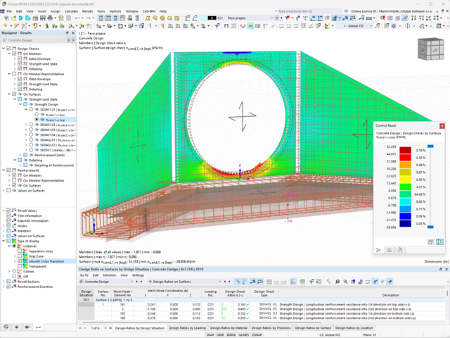
- Graphical output of results integrated in RFEM/RSTAB; for example, design check ratios or required reinforcement
- Numerical results clearly arranged in tables and graphical display of the results in the model
- Integration of the output into the RFEM/RSTAB printout report
- Import of relevant information and results from RFEM
- Integrated, editable material and section library
- Sensible and complete presetting of input parameters
- Punching design on columns (all section shapes), wall ends, and wall corners
- Automatic recognition of the punching node position from an RFEM model
- Detection of curves or splines as a boundary of the control perimeter
- Automatic consideration of all slab openings defined in the RFEM model
- Construction and graphical display of the control perimeter
- Optional design with unsmoothed shear stress along the control perimeter that corresponds to the actual shear stress distribution in the FE model
- Determination of the load increment factor β via full-plastic shear distribution as constant factors according to EN 1992‑1‑1, Sect. 6.4.3 (3), based on EN 1992‑1‑1, Fig. 6.21N, or by a user‑defined specification
- Numerical and graphical display of results (3D, 2D, and in sections)
- Punching design of the slab without punching reinforcement
- Qualitative determination of the required punching reinforcement
- Design and analysis of the longitudinal reinforcement
- Complete integration of results in an RFEM printout report