53 Wyniki
Wyświetl wyniki:
Sortuj według:
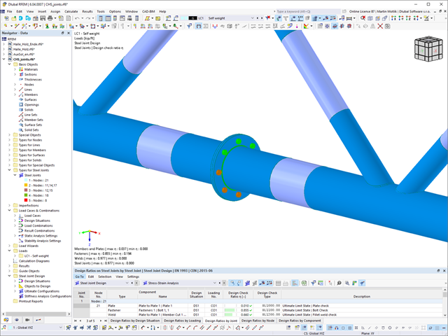
W rozszerzeniu Połączenia stalowe można łączyć profile zamknięte o przekroju okrągłym za pomocą spoin.
Profile okrągłe można łączyć ze sobą lub z płaskimi elementami konstrukcyjnymi. Spoiną można również łączyć pachwiny przekrojów znormalizowanych i cienkościennych.
Przejdź do filmu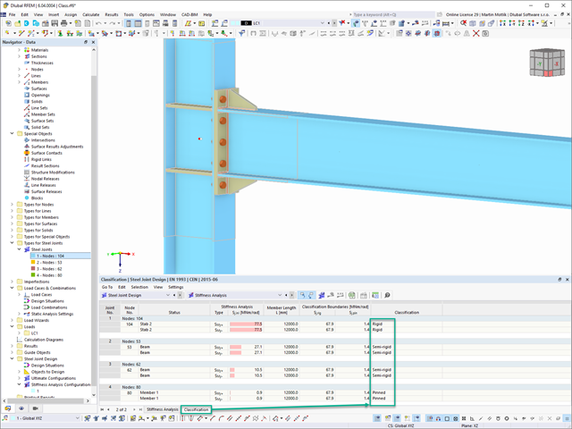
W rozszerzeniu Połączenia stalowe można klasyfikować sztywności połączeń.
Oprócz sztywności początkowej w tabeli wyświetlane są również wartości graniczne dla połączeń przegubowych i sztywnych dla wybranych sił wewnętrznych N, My i/lub Mz. Uzyskana klasyfikacja jest następnie wyświetlana w tabeli jako „przegubowa”, „półsztywna” i „sztywna”.
Przejdź do filmu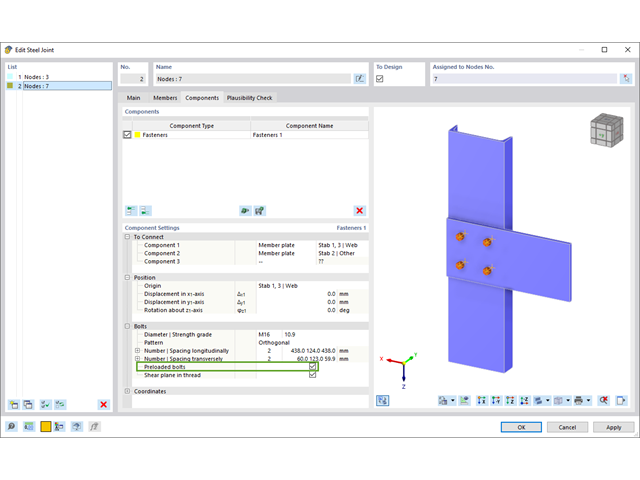
W rozszerzeniu „Połączenia stalowe” można uwzględnić naprężenie wstępne śrub w obliczeniach dla wszystkich komponentów. Sprężenie można łatwo aktywować za pomocą pola wyboru w parametrach śruby i ma ono wpływ zarówno na analizę naprężeniowo-odkształceniową, jak i na analizę sztywności.
Śruby sprężone to specjalne śruby stosowane w konstrukcjach stalowych w celu wygenerowania dużej siły zaciskowej między połączonymi elementami konstrukcyjnymi. Ta siła docisku powoduje tarcie między elementami konstrukcyjnymi, co umożliwia przenoszenie sił.
Funkcjonalność
Śruby sprężane są dokręcane z określonym momentem, co powoduje ich rozciąganie i powstawanie siły rozciągającej. Ta siła rozciągająca jest przenoszona na połączone elementy i prowadzi do powstania dużej siły mocującej. Siła zaciskowa zapobiega poluzowaniu połączenia i zapewnia niezawodne przenoszenie siły.
Zalety
- Wysoka nośność: Śruby wstępnie rozciągane mogą przenosić duże siły.
- Niskie odkształcenie: Minimalizują odkształcenie połączenia.
- Wytrzymałość zmęczeniowa: Są odporne na zmęczenie.
- Łatwość montażu: Są one stosunkowo łatwe w montażu i demontażu.
Analiza i wymiarowanie
Obliczenia śrub sprężanych są przeprowadzane w RFEM z wykorzystaniem modelu analitycznego ES wygenerowanego przez rozszerzenie "Połączenia stalowe". Uwzględnia ona siłę zwarcia, tarcie między elementami konstrukcyjnymi, wytrzymałość śrub na ścinanie oraz nośność elementów konstrukcyjnych. Wymiarowanie odbywa się zgodnie z DIN EN 1993-1-8 (Eurokod 3) lub amerykańską normą ANSI/AISC 360-16. Utworzony model analityczny wraz z wynikami można zapisać i wykorzystać jako niezależny model w programie RFEM.
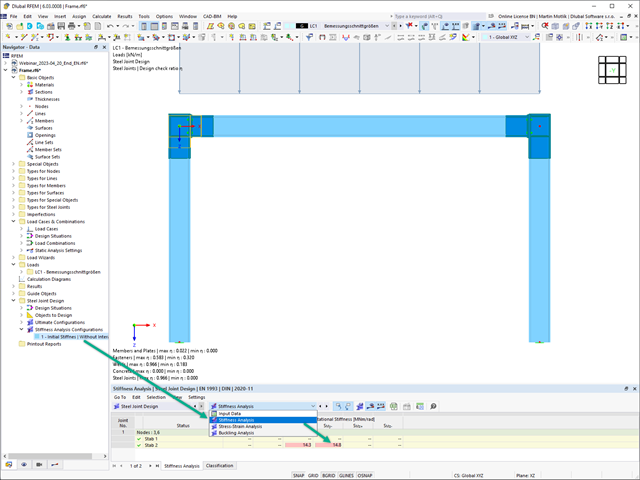
Sztywność początkowa Sj,ini jest parametrem decydującym o ocenie, czy połączenie można scharakteryzować jako sztywne, niesztywne czy przegubowe.
W rozszerzeniu „Połączenia stalowe” można obliczyć początkowe sztywności Sj,ini zgodnie z Eurokodem (EN 1993-1-8 sekcja 5.2.2) i AISC (AISC 360-16 Cl. E3.4) w odniesieniu do sił wewnętrznych N, My i/lub Mz.
Opcjonalne automatyczne przenoszenie sztywności początkowych umożliwia bezpośrednie przenoszenie sztywności przegubowych na końcach prętów w programie RFEM. Następnie cała konstrukcja jest ponownie obliczana, a wynikające z niej siły wewnętrzne są automatycznie uwzględniane jako obciążenia w obliczeniach i wymiarowaniu modeli połączeń.
Ten zautomatyzowany proces iteracji eliminuje konieczność ręcznego eksportu i importu danych, zmniejszając ilość pracy i minimalizując potencjalne źródła błędów.
Film wyjaśniający: Obliczanie sztywności początkowej Sj,ini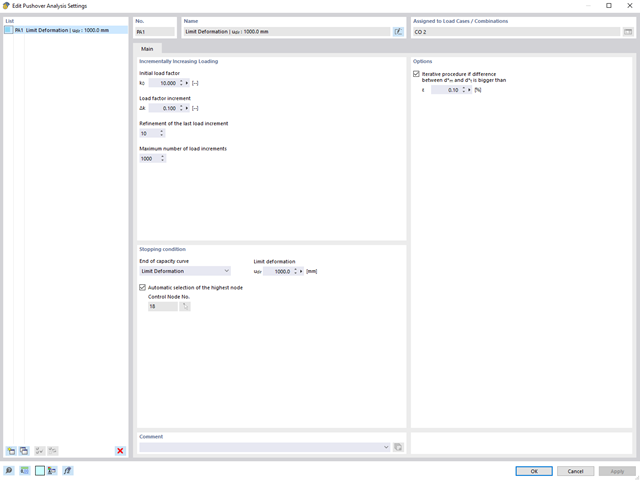
Analiza pushover jest zarządzana przez nowo wprowadzony typ analizy w kombinacjach obciążeń. W tym miejscu można wybrać poziomy rozkład i kierunek obciążenia, obciążenie stałe, żądane spektrum odpowiedzi do określenia docelowego przemieszczenia oraz ustawienia analizy pushover.
W ustawieniach analizy pushover można zmodyfikować przyrost obciążenia poziomego i określić warunek zatrzymania dla analizy. Ponadto użytkownik może bez problemu dostosować precyzyjność iteracyjnego definiowania przesunięcia docelowego.
Rozszerzenie Połączenia stalowe umożliwia wymiarowanie połączeń prętów o złożonych przekrojach. Ponadto można przeprowadzać obliczenia połączeń dla prawie wszystkich przekrojów cienkościennych z biblioteki programu RFEM.
Przejdź do filmu
W rozszerzeniu Połączenia stalowe można wymiarować połączenia zgodnie z amerykańską normą ANSI/AISC 360-16. Zintegrowane zostały następujące metody obliczeń:
- Obliczenia współczynnika obciążenia i odporności (LRFD)
- Projektowanie dopuszczalnych naprężeń (ASD)
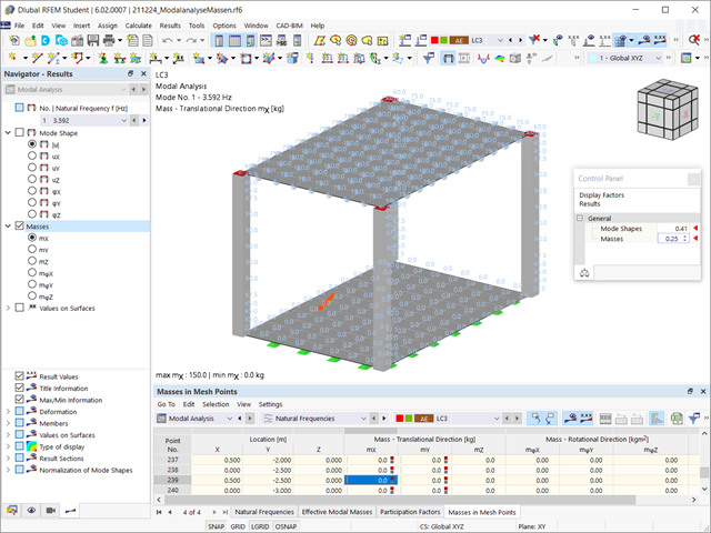
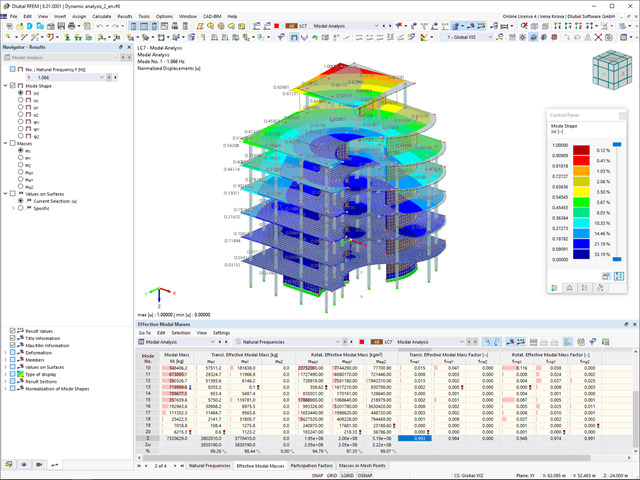
Czy odkryłeś już tabelaryczne i graficzne przedstawianie mas w punktach siatki? Po prawej, jest to również jeden z wyników analizy modalnej w programie RFEM 6. W ten sposób można sprawdzić importowane masy, które zależą od różnych ustawień analizy modalnej. Mogą być one wyświetlane w zakładce Masy w punktach siatki tabeli Wyniki. Tabela zawiera przegląd następujących wyników: Masa - kierunek przesuwny (mX, mY, mZ ), Masa - kierunek obrotowy (mφX, mφY, mφZ ) oraz suma mas. Czy nie byłoby lepiej, gdybyś jak najszybciej przeprowadził ocenę graficzną? Następnie można również wyświetlić graficznie masy w punktach siatki.
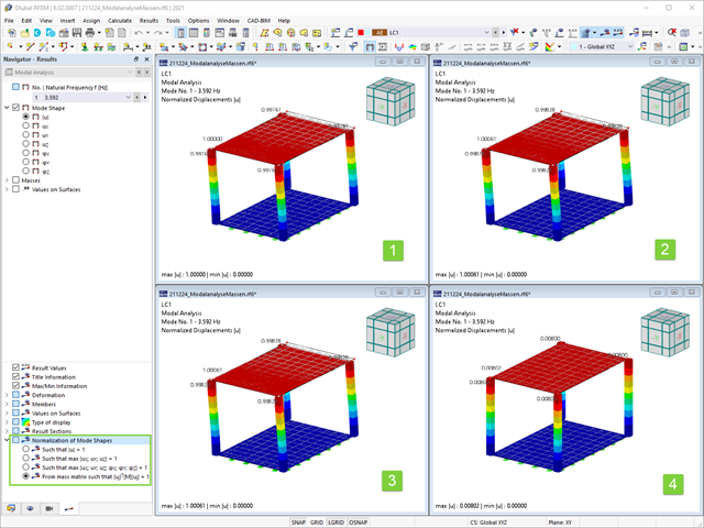
Jak już wiesz, po pomyślnym zakończeniu obliczeń wyniki przypadku obciążenia w Analizie modalnej są wyświetlane w programie. Die erste Eigenform ist für Sie also sofort grafisch oder animiert zu sehen. Dabei können Sie die Darstellung der Eigenformnormierung komfortabel anpassen. Erledigen Sie das am besten direkt im Ergebnisnavigator, wo Sie zur Visualisierung der Eigenformen eine von vier Optionen auswählen:
- Wert des Eigenformvektors uj auf 1 skalieren (berücksichtigt nur die Translationskomponenten)
- Auswahl der maximalen Translationskomponente des Eigenvektors und Einstellung auf 1
- Betrachtung der gesamten Eigenform (inklusive der Rotationskomponenten), Auswahl des Maximums und Einstellung auf 1
- Setzen der modalen Massen mi für jeden Eigenwert auf 1 kg
Ausführlichere Erläuterungen der Normierung der Eigenformen finden Sie hier: Instrukcja online .
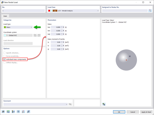
Czy oprócz obciążeń statycznych chcesz uwzględnić również inne obciążenia jako masy? Program umożliwia to dla obciążeń węzłowych, prętowych, liniowych i powierzchniowych. W tym celu podczas definiowania obciążenia należy wybrać typ Obciążenie masą. Dla takich obciążeń należy zdefiniować masę lub składowe masy w kierunkach X, Y i Z. W przypadku mas węzłowych można dodatkowo zdefiniować momenty bezwładności X, Y i Z w celu modelowania bardziej złożonych punktów mas.
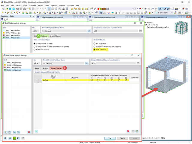
Często zachodzi potrzeba pominięcia mas. Dzieje się tak zwłaszcza w przypadku, gdy wyniki analizy modalnej mają być wykorzystane do analizy sejsmicznej. W tym celu wymagane jest 90% efektywnej masy modalnej w każdym kierunku. Pozwala to na pominięcie masy we wszystkich utwierdzonych podporach węzłowych i liniowych. Program automatycznie dezaktywuje powiązane masy.
Obiekty, których masy mają zostać pominięte w analizie modalnej, można również wybrać ręcznie. Dla lepszego widoku pokazaliśmy to ostatnie na rysunku. W wyniku wyboru przez użytkownika obiektów masowych wraz z skojarzonymi z nimi składowymi masowymi można pominąć masy.
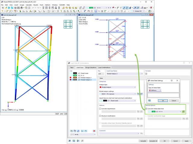
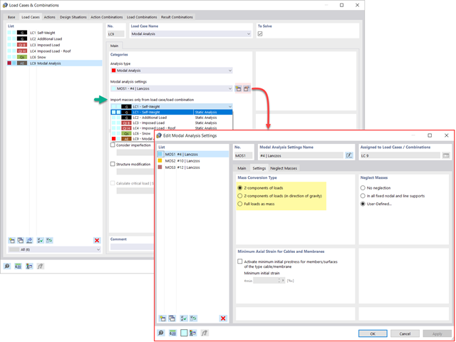
Podczas definiowania danych wejściowych dla przypadku obciążenia analizy modalnej można uwzględnić przypadek obciążenia, którego sztywności reprezentują początkową pozycję analizy modalnej. Jak to zrobić? Jak pokazano na rysunku, należy wybrać opcję "Uwzględnij stan początkowy z". Teraz otwórz okno dialogowe "Ustawienia stanu początkowego" i zdefiniuj typ Sztywność jako stan początkowy. W tym przypadku obciążenia, który jest stanem początkowym branym pod uwagę, można uwzględnić sztywność układu konstrukcyjnego, gdy pręty rozciągane ulegają uszkodzeniu. Celem tego wszystkiego: Sztywność z tego przypadku obciążenia jest uwzględniana w analizie modalnej. W ten sposób uzyskuje się wyraźnie elastyczny system.
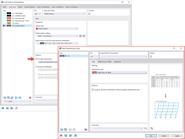
Widać to już na obrazku: Imperfekcje można również uwzględnić podczas definiowania przypadku obciążenia w analizie modalnej. Typy imperfekcji, które mogą być stosowane w analizie modalnej, to obciążenia hipotetyczne z przypadku obciążenia, początkowe przemieszczenie w tabeli, odkształcenie statyczne, postać wyboczeniowa, postać dynamiczna oraz grupa przypadków imperfekcji.
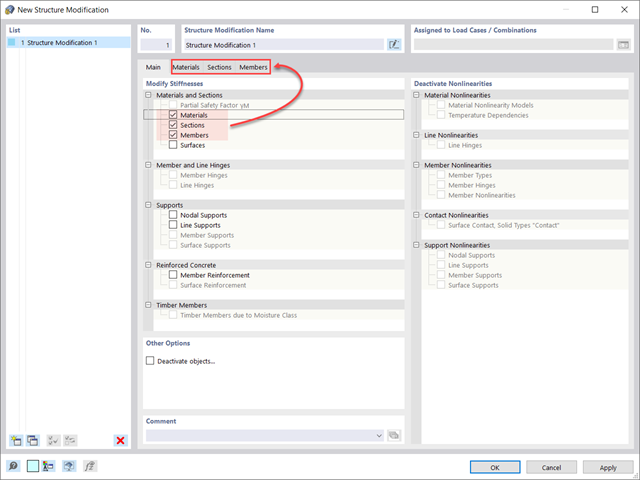
Czy wiecie, że...? W przypadkach obciążeń typu Analiza modalna można z łatwością wprowadzać zmiany konstrukcyjne. Pozwala to na przykład na indywidualne dostosowanie sztywności materiałów, przekrojów, prętów, powierzchni, przegubów i podpór. W przypadku niektórych rozszerzeń można również modyfikować sztywności. Po wybraniu obiektów ich właściwości sztywności są dostosowywane do typu obiektu. W ten sposób można je zdefiniować w osobnych zakładkach.
Czy chcesz przeanalizować uszkodzenie obiektu (na przykład słupa) w analizie modalnej? Jest to również możliwe bez żadnych problemów. Wystarczy przejść do okna Modyfikacja konstrukcji i dezaktywować odpowiednie obiekty.
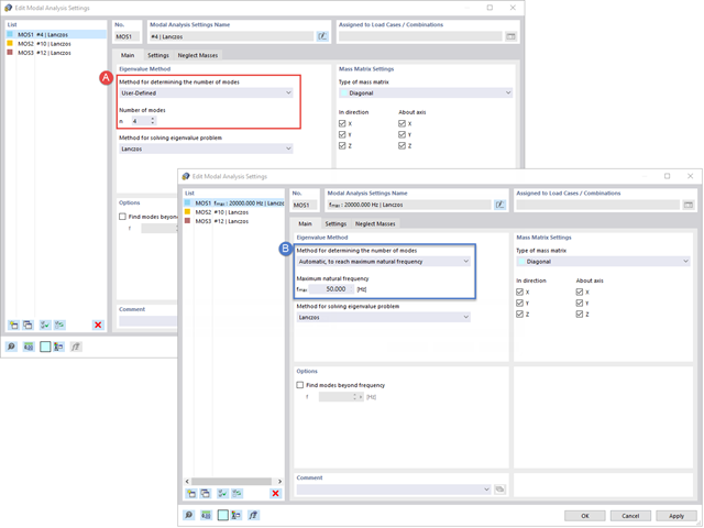
Twoim celem jest określenie liczby postaci drgań własnych? Program oferuje dwie metody. Z jednej strony, można ręcznie zdefiniować liczbę najmniejszych kształtów drgań, które mają zostać obliczone. W tym przypadku liczba dostępnych kształtów postaci zależy od stopni swobody (tzn. liczby punktów mas swobodnych pomnożonych przez liczbę kierunków, w których działają masy). Jest to jednak ograniczone do 9999. Z drugiej strony, maksymalną częstotliwość drgań własnych można ustawić w taki sposób, w jaki program określił kształty automatycznie, aż do osiągnięcia zadanej częstotliwości drgań własnych.
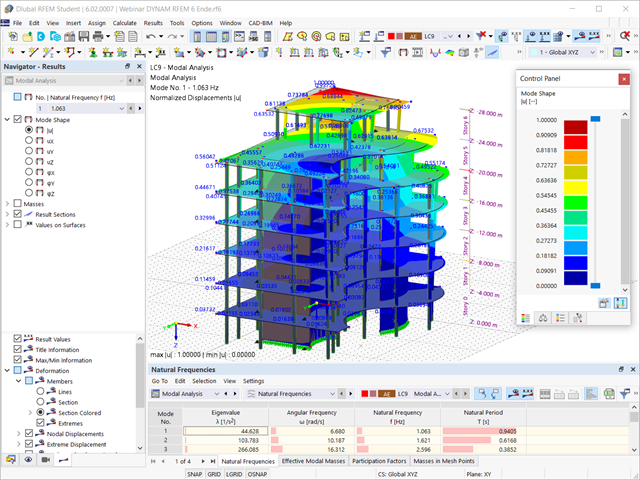
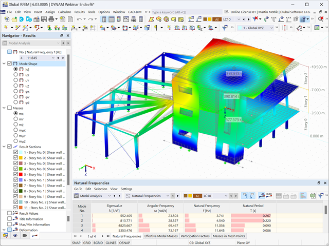
Czy obliczenia się zakończyły? Wyniki analizy modalnej są wówczas dostępne zarówno w formie graficznej, jak i tabelarycznej. Wyświetl tabele wyników dla przypadku obciążenia lub przypadków obciążeń analizy modalnej. Dzięki temu na pierwszy rzut oka można zobaczyć wartości własne, częstotliwości kątowe, częstotliwości i okresy drgań własnych konstrukcji. W przejrzysty sposób wyświetlane są również efektywne masy modalne, modalne współczynniki masy i współczynniki udziału.
Dostępnych jest kilka opcji definiowania mas dla analizy modalnej. Masy od ciężaru własnego są uwzględniane automatycznie, natomiast obciążenia i masy można uwzględnić bezpośrednio w przypadku obciążenia typu analiza modalna. Potrzebujesz więcej opcji? Należy wybrać, czy obciążenia pełne mają być uwzględniane jako masy, składowe obciążenia w globalnym kierunku Z, czy tylko składowe obciążenia w kierunku siły ciężkości.
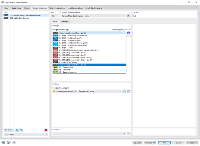
Program oferuje dodatkową lub alternatywną opcję importu mas: Ręczna definicja kombinacji obciążeń, począwszy od których masy są uwzględniane w analizie modalnej. Wybrałeś normę obliczeniową? Następnie można utworzyć sytuację obliczeniową typu Kombinacja mas sejsmicznych. W ten sposób program automatycznie oblicza sytuację masową dla analizy modalnej zgodnie z preferowaną normą obliczeniową. Innymi słowy: Program tworzy kombinację obciążeń na podstawie współczynników kombinacji wstępnie ustawionych dla wybranej normy. Zawiera on masy użyte do analizy modalnej.
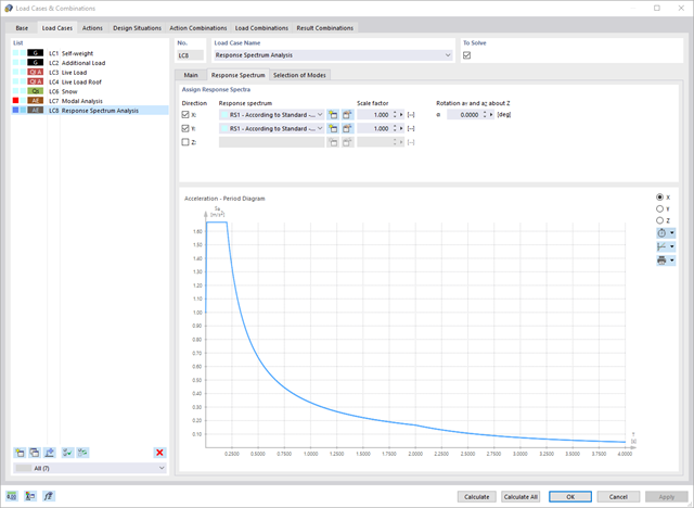
Oprogramowanie do analizy statyczno-wytrzymałościowej firmy Dlubal wykonuje wiele pracy za Ciebie. Program sugeruje zgodnie z regułami parametry wejściowe, istotne dla wybranych norm. Ponadto można ręcznie wprowadzić spektra odpowiedzi.
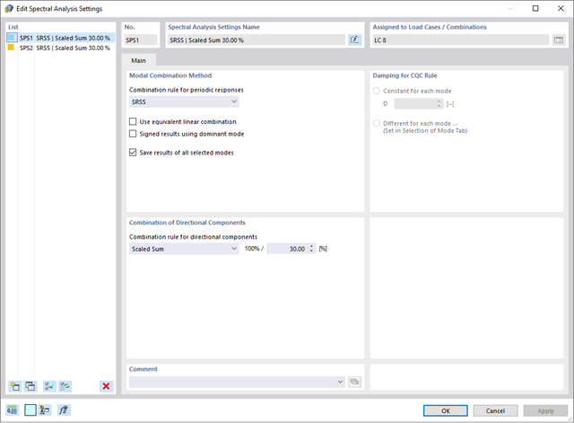
Przypadki obciążeń typu Analiza spektrum odpowiedzi określają kierunek, w którym działają spektra odpowiedzi oraz które wartości własne konstrukcji są istotne dla analizy. W ustawieniach analizy spektralnej można zdefiniować szczegóły dotyczące reguł kombinacji, tłumienia (jeśli ma zastosowanie) i przyspieszenia okresu zerowego (ZPA).
Czy wiecie, że...? Równoważne obciążenia statyczne generowane są oddzielnie dla każdej miarodajnej postaci drgań własnych oraz kierunku wzbudzenia. Obciążenia te są zapisywane w przypadku obciążenia typu Analiza spektrum odpowiedzi, a program RFEM/RSTAB przeprowadza liniową analizę statyczną.
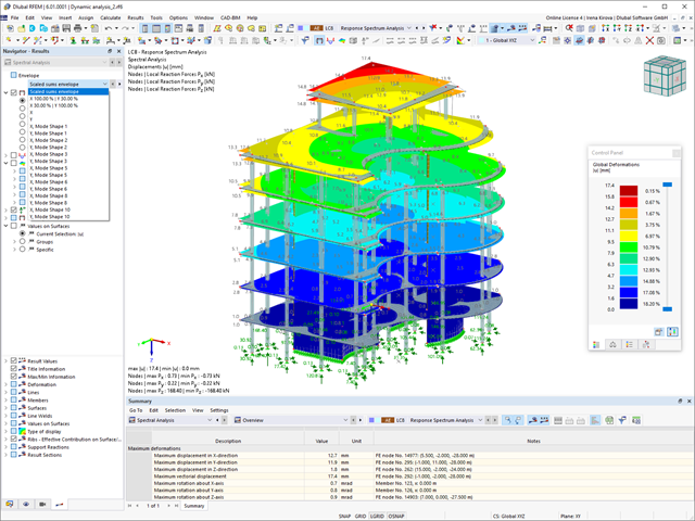
Przypadki obciążeń typu Analiza spektrum odpowiedzi zawierają wygenerowane obciążenia równoważne. Po pierwsze, udziały modalne muszą zostać nałożone na siebie z regułą SRSS lub CQC. W takim przypadku można wykorzystać wyniki podpisane na podstawie dominującego kształtu drgań.
Następnie składowe kierunkowe oddziaływań sejsmicznych są łączone z regułą SRSS lub regułą 100%/30%.
- Automatyczne uwzględnianie masy własnej od ciężaru konstrukcji
- Możliwy bezpośredni import mas z przypadków obciążeń lub kombinacji
- Opcjonalne definiowanie mas dodatkowych (masy węzłowe, liniowe lub powierzchniowe oraz masy wynikające z bezwładności) bezpośrednio w przypadkach obciążeń
- Opcjonalne pominięcie mas (na przykład masy fundamentów)
- Kombinacje mas w różnych przypadkach i kombinacjach obciążeń
- Predefiniowane współczynniki kombinacji wg różnych norm (EC 8, SIA 261, ASCE 7, ...)
- Opcjonalny import stanów początkowych (np. w celu uwzględnienia naprężenia wstępnego i imperfekcji)
- modyfikacja konstrukcji
- Uwzględnianie uszkodzenia w podporach lub prętach/powierzchniach/bryłach
- Możliwość zadania kilku analiz modalnych (np. w celu analizy różnych mas lub modyfikacji sztywności)
- Wybór typu macierzy mas (macierz diagonalna, macierz spójna, macierz jednostkowa) oraz wskazanych przez użytkownika stopni swobody (translacyjne i rotacyjne)
- Metody określania liczby postaci drgań własnych (liczba zdefiniowana przez użytkownika, liczba określana automatycznie - w celu osiągnięcia zadanych efektywnych współczynników masy modalnej, liczba określana automatycznie - w celu osiągnięcia maksymalnej częstotliwości drgań własnych - dostępne tylko w programie RSTAB)
- Określanie postaci drgań i mas w węzłach siatki MES
- Wyniki w postaci wartości własnych, częstości kątowych, częstotliwości drgań własnych i okresu drgań własnych
- Wyniki w postaci mas modalnych, efektywnych mas modalnych, współczynników masy modalnej i współczynników udziału masy
- Tabelaryczne i graficzne przedstawienie mas w punktach siatki MES
- Wizualizacja i animacja postaci drgań własnych
- Różne opcje skalowania postaci drgań własnych
- Dokumentacja wyników numerycznych i graficznych w raporcie
W ustawieniach analizy modalnej należy wprowadzić wszystkie dane, które są niezbędne do określenia częstotliwości drgań własnych. Są to na przykład kształty mas i solwery wartości własnych.
Rozszerzenie Analiza modalna określa najniższe wartości częstości drgań własnych konstrukcji. Liczbę wartości własnych można dostosować lub określić automatycznie. Należy zatem osiągnąć efektywne współczynniki masy modalnej lub maksymalne częstotliwości drgań własnych. Masy są importowane bezpośrednio z przypadków obciążeń i kombinacji obciążeń. W takim przypadku istnieje możliwość uwzględnienia masy całkowitej, składowych obciążenia w globalnym kierunku Z lub tylko składowej obciążenia w kierunku siły ciężkości.
Dodatkowe masy w węzłach, liniach, prętach lub powierzchniach można zdefiniować ręcznie. Ponadto można wpływać na macierz sztywności poprzez import sił osiowych lub modyfikacji sztywności z przypadku obciążenia lub kombinacji obciążeń.
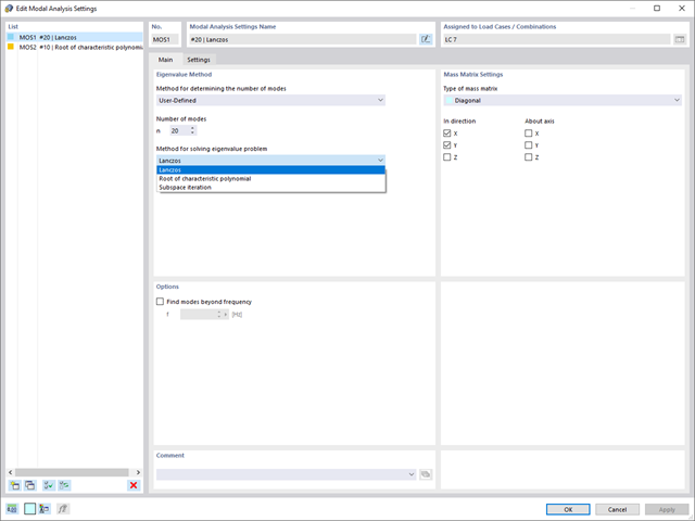
W programie RFEM dostępne są trzy wydajne solwery wartości własnych:
- pierwiastek wielomianu charakterystycznego
- Metoda Lanchosa
- iteracja podprzestrzeni
Z kolei program RSTAB oferuje dwa solwery wartości własnych:
- iteracja podprzestrzeni
- Metoda Powera z przesuniętą odwrotnością
Wybór solwera wartości własnych zależy przede wszystkim od rozmiaru modelu.
Zaraz po zakończeniu obliczeń wyświetlane są wartości własne, częstotliwości drgań własnych i okresy. Okna z tymi wynikami zintegrowane są z programem głównym RFEM/RSTAB. W tabelach można znaleźć wszystkie kształty drgań konstrukcji, a także można je wyświetlić graficznie i animować.
Wszystkie tabele wyników i grafiki stanowią część raportu programu RFEM/RSTAB. Zapewnia to przejrzystą dokumentację obliczeń. Tabele można również eksportować do programu MS Excel.
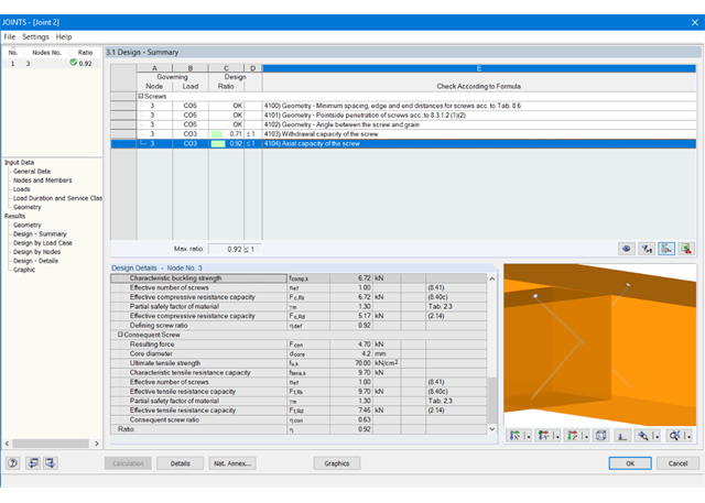
Główne funkcje wymiarowania połączeń są najpierw pogrupowane i wyświetlane wraz z podstawową geometrią połączenia w pierwszym oknie wyników. W kolejnych oknach wyników można zobaczyć wszystkie istotne szczegóły obliczeń.
Wymiary, właściwości materiału i spoiny istotne dla konstrukcji połączenia są wyświetlane natychmiast i można je wydrukować. Podobnie aktywowany jest eksport do pliku DXF. Połączenia można zwizualizować w module RF-/JOINTS Timber - Timber to Timber oraz w programie RFEM/RSTAB.
Wszystkie grafiki mogą zostać dołączone do protokołu wydruku programu RFEM/RSTAB lub wydrukowane bezpośrednio. Dzięki skalowaniu wyników, możliwa jest optymalna kontrola wizualna już na etapie projektowania.
Moduł wyświetla następujące wyniki:
- Minimalna odległość między trzpieniami
- Nośność każdego wkręta
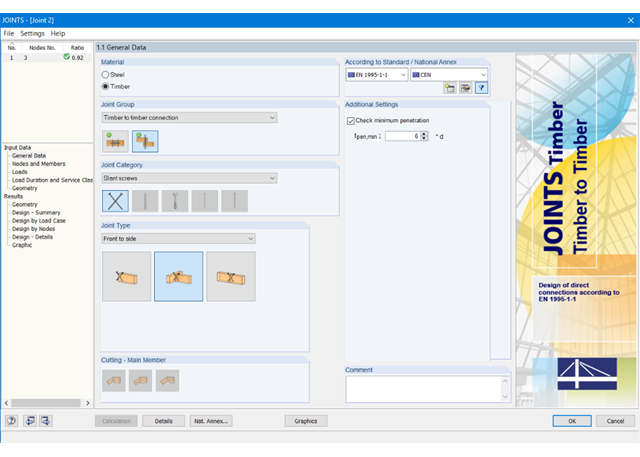
Najpierw należy wybrać typ połączenia i normę obliczeniową.
Połączone pręty są importowane z modelu w programie RFEM/RSTAB. Moduł dodatkowy automatycznie sprawdza, czy wszystkie warunki geometrii są spełnione.
Ponadto obciążenia są importowane automatycznie z programu RFEM/RSTAB. W oknie Geometria można określić parametry wkręta (średnica, długość, kąt itp.).
.png?mw=640&hash=c1087880acc023575381bb136280b0c348568350)
- Obliczanie połączeń przegubowych
- Nachylenie dwuosiowe połączonego pręta (np. połączenie krokwi)
- Połączenie dowolnej liczby prętów na jednym węźle dla typu "Tylko pręt główny"
- Średnica wkręta 6 mm - 12 mm
- Automatyczne sprawdzanie minimalnego rozstawu wkrętów
- Optymalne definiowanie rozstawu wkrętów
- Przenoszenie mimośrodu z RFEM/RSTAB
- Poprzeczne lub równoległe rozmieszczenie wkrętów
- Zdefiniowanie do 16 wkrętów w rzędzie
- Graficzne przedstawienie połączeń w module dodatkowym i w RFEM/RSTAB
- Możliwość przeprowadzenia wszystkich wymaganych obliczeń
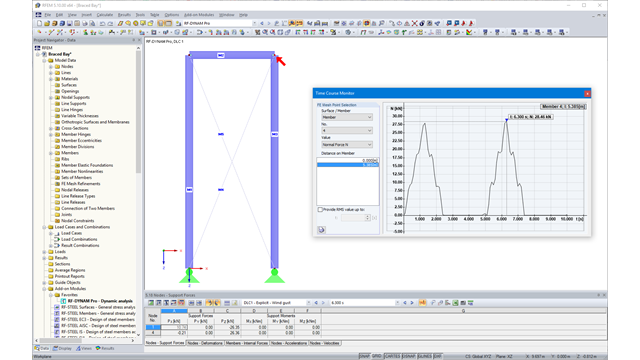
Dzięki integracji RF-/DYNAM Pro z programem RFEM lub RSTAB, do globalnego raportu można włączać numeryczne i graficzne wyniki z RF-/DYNAM Pro - Nonlinear Time History. Ponadto wszystkie opcje w programach RFEM i RSTAB są dostępne do wizualizacji graficznej. Wyniki analizy przebiegu czasowego wyświetlane są na wykresie przebiegu czasowego.
Wyniki są wyświetlane w funkcji czasu, a wartości liczbowe można eksportować do programu MS Excel. Kombinacje wyników mogą być eksportowane jako wynik pojedynczego kroku czasowego lub najbardziej niekorzystne wyniki wszystkich kroków czasowych są odfiltrowywane.
Obliczenia w RFEM
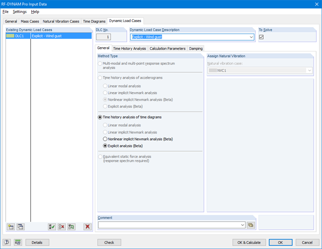
Nieliniowa analiza przebiegu czasowego jest przeprowadzana za pomocą pośredniej analizy Newmarka lub analizy bezpośredniej. Obie metody są metodami bezpośredniej integracji czasu. Analiza pośrednia wymaga definiowania małych kroków czasowych w celu dostarczenia dokładnych wyników. Analiza bezpośrednia określa automatycznie wymagany krok czasowy, w celu zapewnienia stabilności rozwiązania. Analizę bezpośrednią stosuje się w przypadku obliczania krótkotrwałych wzbudzeń, takich jak wzbudzenia impulsowe lub wybuch.
Obliczenia w RSTAB
Nieliniowa analiza przebiegu czasowego jest przeprowadzana z wykorzystaniem analizy bezpośredniej. Jest to metoda bezpośredniej integracji czasu i określa automatycznie krok czasowy, konieczny w celu zapewnienia stabilności wyników obliczeń.