14 Wyniki
Wyświetl wyniki:
Sortuj według:
- 002089
- Ogólne informacje
- Skręcanie skrępowane (7 stopni swobody) RFEM 6
- Skręcanie skrępowane (7 stopni swobody) RSTAB 9
- Uwzględnienie 7 lokalnych kierunków deformacji (ux , uy, uz, φx, φy, φz, ω ) lub 8 sił wewnętrznych (N , Vu, Vv, Mt, pri, Mt, s, Mu, Mv, Mω ) przy obliczaniu elementów prętowych
- Możliwość stosowania w połączeniu z analizą statyczno-wytrzymałościową według teorii II rzędu, i analiza dużych deformacji (można również uwzględnić imperfekcje)
- W połączeniu z rozszerzeniem Analiza stateczności umożliwia definiowanie współczynników obciążenia krytycznego i kształtów drgań dla problemów stateczności, takich jak wyboczenie skrętne i zwichrzenie
- Uwzględnianie blach czołowych i usztywnień poprzecznych jako sprężystości skrępowanej podczas obliczania przekrojów dwuteowych z automatycznym określaniem i wyświetlaniem graficznym sztywności sprężystości deplanacyjnej
- Graficzne przedstawienie deplanacji przekroju prętów w stanie odkształcenia
- Pełna integracja z RFEM i RSTAB

- 002090
- Ogólne informacje
- Skręcanie skrępowane (7 stopni swobody) RFEM 6
- Skręcanie skrępowane (7 stopni swobody) RSTAB 9
Obliczenia skręcania skrępowanego można przeprowadzić dla całego układu. Uwzględniasz zatem dodatkową wartość 7 stopnia swobody w obliczeniach pręta. Sztywności połączonych elementów konstrukcyjnych są uwzględniane automatycznie. Oznacza to, że nie ma potrzeby' definiowania równoważnych sztywności sprężystych ani warunków podparcia dla układu odłączanego.
Następnie można wykorzystać siły wewnętrzne z obliczeń ze skręcaniem skrępowanym w rozszerzeniu do obliczeń. W zależności od materiału i wybranej normy należy uwzględnić bimoment wyboczeniowy i drugorzędny moment skręcający. Typowym zastosowaniem jest analiza stateczności według teorii drugiego rzędu z wykorzystaniem imperfekcji w konstrukcjach stalowych.
Czy wiecie, że...? Zastosowanie nie ogranicza się do przekrojów stalowych cienkościennych. Pozwala to na przykład na przeprowadzenie obliczeń idealnego momentu krytycznego dla belek o przekrojach z drewna litego.
- 002401
- Ogólne informacje
- Skręcanie skrępowane (7 stopni swobody) RFEM 6
- Skręcanie skrępowane (7 stopni swobody) RSTAB 9
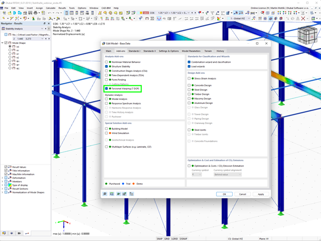
- Funkcję skręcania skrępowanego można aktywować lub dezaktywować w zakładce Rozszerzenia w Danych podstawowych modelu.
- Po aktywowaniu rozszerzenia interfejs użytkownika w programie RFEM zostaje rozszerzony o nowe wpisy w nawigatorze, tabelach i oknach dialogowych.
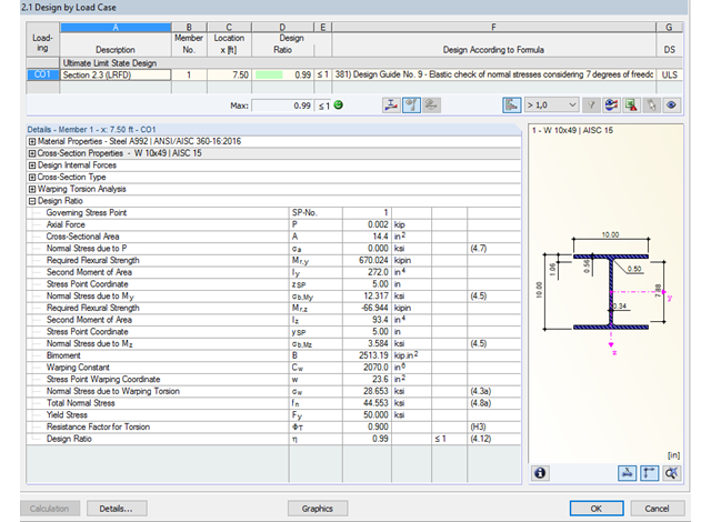
Dzięki zintegrowanemu rozszerzeniu modułu RF-/STEEL Warping Torsion, możliwe jest przeprowadzenie obliczeń zgodnie z Design Guide 9 w RF-/STEEL AISC.
Obliczenia są przeprowadzane z 7 stopniami swobody zgodnie z teorią skręcania skrępowanego i umożliwiają realistyczne obliczenia stateczności z uwzględnieniem skręcania.
Definiowanie krytycznego momentu wyboczeniowego odbywa się w module RF-/STEEL AISC za pomocą solwera wartości własnych, który umożliwia dokładne określenie krytycznego obciążenia wyboczeniowego.
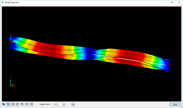
Solwer wartości własnych pokazuje okno z grafiką wartości własnych, które umożliwia sprawdzenie warunków brzegowych.
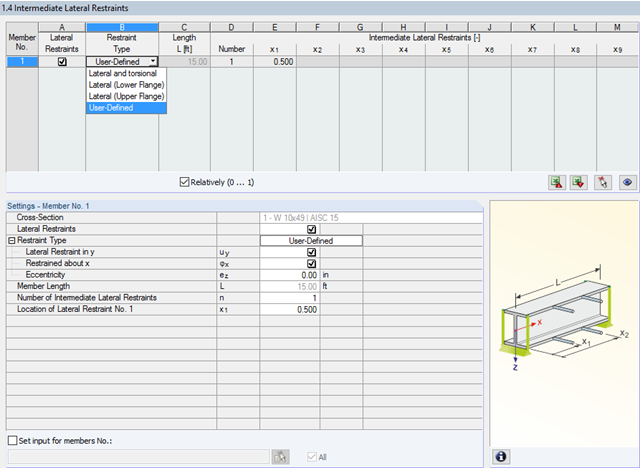
W programie STEEL AISC możliwe jest uwzględnienie pośrednich podpór bocznych w dowolnym miejscu. Na przykład, możliwa jest stabilizacja tylko górnej półki.
Ponadto można przypisać boczne podpory pośrednie zdefiniowane przez użytkownika; na przykład pojedyncze sprężyny obrotowe i sprężyny translacyjne w dowolnym miejscu przekroju.
- Modelowanie przekroju za pomocą elementów, profili, łuków i elementów punktowych
- Biblioteka właściwości materiałów, granic plastyczności i naprężeń granicznych, którą użytkownik może rozbudowywać
- Właściwości przekrojów otwartych, zamkniętych i niepołączonych
- Efektywne właściwości przekrojów wykonanych z różnych materiałów
- Określanie naprężeń w spoinach pachwinowych
- Analiza naprężeń wraz z obliczaniem skręcania swobodnego i skrępowanego
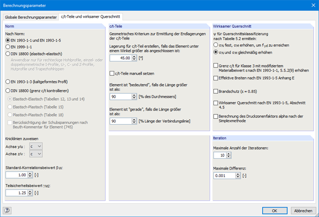
- Sprawdzanie stosunków (c/t)
- Przekroje efektywne według
- EN 1993-1-5 (w tym płyty usztywnione zgodnie z rozdziałem 4.5)
-
 EN 1993-1-3
 -
EN 1999-1-1
-
 DIN 18800-2
- Klasyfikacja według
-
EN 1993-1-1
-
EN 1999-1-1
-
- Interfejs z MS Excel służący do importu i eksportu tabel
- Raport
- Stosuje się do prętów zdefiniowanych jako zbiory prętów
- Oddzielny solwer uwzględniający 7 kierunków deformacji (ux , uy, uz, φx, φy, φz, ω ) lub 8 sił wewnętrznych (N, Vu, Vv, Mt, pri, Mt, s, Mu, Mv,M )
- Projektowanie nieliniowe według analizy drugiego rzędu
- Wprowadzanie imperfekcji
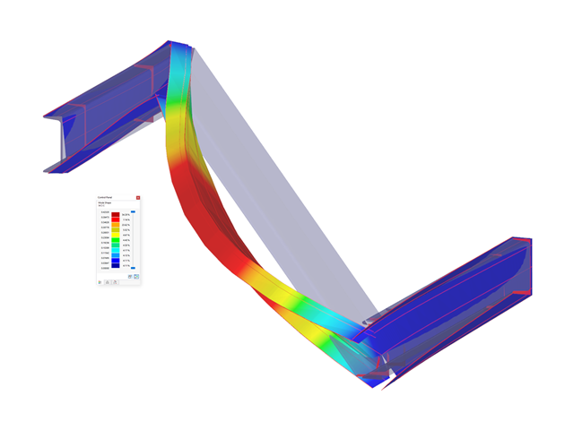
- Obliczanie współczynników obciążenia krytycznego i postaci wyboczenia oraz ich wizualizacja (wraz z skręcaniem skrępowanym)
- Integracja z wymiarowaniem prętów w modułach dodatkowych RF-/STEEL AISC i RF-/STEEL EC3
- Dostępne dla wszystkich przekrojów stalowych cienkościennych
Wszystkie wyniki mogą być wyświetlane i analizowane w postaci numerycznej i graficznej. W przypadku wizualizacji wyników, narzędzia wyboru pozwalają na ich szczegółową ocenę.
Protokół wydruku spełnia wysokie standardy Produkt | RFEM 6 und des Produkt | RSTAB 9 . Modyfikacje przekroju aktualizowane są automatycznie.
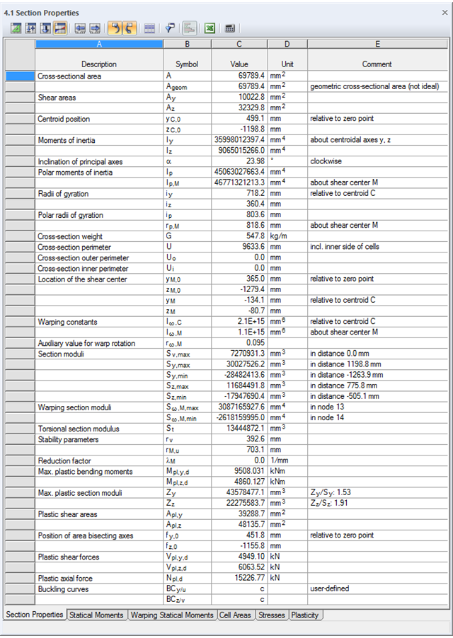
SHAPE-THIN określa wszystkie odpowiednie charakterystyki przekroju, wraz z plastycznymi siłami granicznymi i momentami. Nakładające się powierzchnie są uwzględniane w sposób realistyczny. Dla przekrojów utworzonych z różnych materiałów, SHAPE-THIN określa idealne charakterystyki przekroju w odniesieniu do materiału referencyjnego.
Oprócz analizy naprężeń w stanie sprężystym, można prowadzić również obliczenia w stanie plastycznym, zawierające interakcję sił wewnętrznych dla różnorodnych kształtów przekroju. Obliczenia interakcji plastycznej prowadzane są według metody Simplex. Podczas analizy naprężeń można wybrać różne teorie (Tresca lub von Mises).
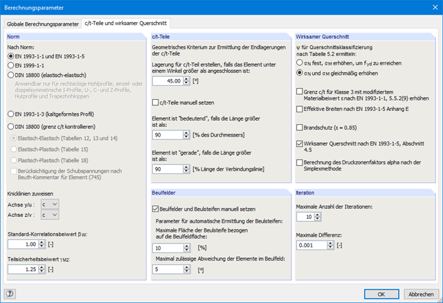
SHAPE-THIN przeprowadza klasyfikację przekroju zgodnie z EN 1993-1-1 i EN 1999-1-1. W przypadku przekrojów stalowych o przekroju 4, program określa szerokości efektywne dla płyt usztywnionych lub nieusztywnionych, zgodnie z EN 1993-1-1 i EN 1993-1-5. W przypadku przekrojów aluminiowych o przekroju klasy 4, program oblicza grubości efektywne zgodnie z EN 1999-1-1.
Opcjonalnie SHAPE-THIN sprawdza wartości graniczne c/t zgodnie z metodami obliczeniowymi el-el, el-pl lub pl-pl zgodnie z DIN 18800. Przekrój jest klasyfikowany według danej kombinacji sił wewnętrznych.
SHAPE-THIN posiada obszerną bibliotekę przekrojów walcowanych i parametryzowanych. Mogą one być łączone lub uzupełniane o nowe elementy. Możliwe jest zamodelowanie przekroju składającego się z różnych materiałów.
Narzędzia i funkcje graficzne umożliwiają modelowanie złożonych kształtów przekrojów w sposób typowy dla programów CAD. W oknie graficznym można wprowadzić elementy punktowe, spoiny pachwinowe, łuki, sparametryzowane przekroje prostokątne i okrągłe, elipsy, łuki eliptyczne, parabole, hiperbole, splajn oraz NURBS. Alternatywnie można zaimportować plik DXF, który stanowi podstawę do dalszego modelowania. Podczas modelowania można użyć także linii pomocniczych.
Ponadto, sparametryzowane wprowadzanie danych umożliwia wprowadzanie danych modelu i obciążeń w określony sposób, tak aby były one zależne od określonych zmiennych.
Elementy można graficznie podzielić lub przydzielić do innych obiektów. SHAPE-THIN automatycznie dzieli elementy i zapewnia nieprzerwany przepływ ścinający poprzez wprowadzenie elementów zerowych. W przypadku elementów zerowych można zdefiniować określoną grubość, aby kontrolować przenoszenie ścinania.
SHAPE-THIN określa charakterystyki przekroju i naprężenia dla przekrojów otwartych, zamkniętych, połączonych i niepołączonych.
- parametry przekroju
- Pole przekroju A
- Pole ścinane Ay, Az, Au i Av
- Położenie środka ciężkości yS, zS
- momenty pola 2 stopnie Iy, Iz, Iyz, Iu, Iv, Ip, Ip,M
- Promienie bezwładności iy, iz, iyz, iu, iv, ip, ip,M
- Nachylenie osi głównych α
- Ciężar przekroju G
- Średnica przekroju U
- momenty bezwładności przy skręcaniu stopnieIT , IT , IT,St.Venant, IT,Bredt, IT,s
- Położenie środka ścinania yM, zM
- Stałe deplanacji Iω,S, Iω,M or Iω,D dla utwierdzenia bocznego
- Max/min moduły przekroju Sy, Sz, Su, Sv, Sω,M z położeniami
- Promienie przekroju ru, rv, rM,u, rM,v
- Współczynnik redukcyjny λM
- Plastyczne charakterystyki przekroju
- Siła osiowa Npl,d
- Siły tnące Vpl,y,d, Vpl,z,d, Vpl,u,d, Vpl,v,d
- Momenty zginające Mpl,y,d, Mpl,z,d, Mpl,u,d, Mpl,v,d
- Moduły przekroju Zy, Zz, Zu, Zv
- Pola ścinania Apl,y, Apl,z, Apl,u, Apl,v
- Położenie osi powierzchni fu, fv,
- Wyświetlanie elipsy bezwładności
- Momenty statyczne pola Qu, Qv, Qy, Qz z położeniem maksimum i określeniem przebiegu ścinania
- Współrzędne wycinkowe ωM
- momenty bezwładności (wycinkowe powierzchnie) Sω,M
- Pola komórek Am zamkniętych przekrojów
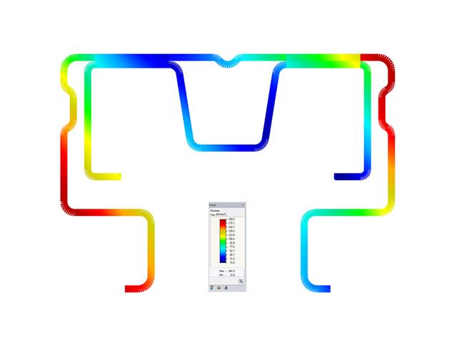
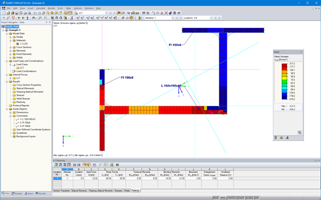
- Naprężenia normalne σx wywołane siłą osiową, momentem zginającym i bimomentem deplanacji
- Naprężenia styczne τ od sił tnących oraz pierwotnych i drugorzędnych momentów skręcających
- Naprężenia zastępcze σv ze współczynnikiem dla naprężeń ścinających, który można dostosować do własnych potrzeb
- Stopnie wykorzystania odniesione do naprężeń granicznych
- Naprężenia dla krawędzi lub osi elementu
- Naprężenia w spoinach pachwinowych
- Charakterystyki przekrojów niepołączonych (rdzeń budynku wysokościowego, przekroje złożone)
- Siły tnące wywołane zginaniem i skręcaniem
- Obliczanie nośności plastycznej z określeniem współczynnika zwiększającego αpl
- Sprawdzenie stosunków c/t według metody el-el, el-pl lub pl-pl wg DIN 18800
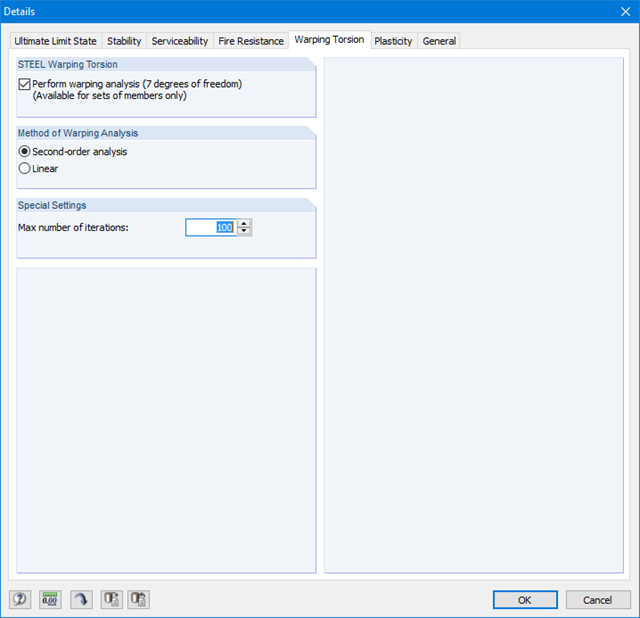
Ponieważ moduł RF-/STEEL Warping Torsion jest w pełni zintegrowany z modułami RF-/STEEL AISC i RF‑/STEEL EC3, dane są wprowadzane w taki sam sposób, jak w przypadku obliczeń w tych modułach. W oknie dialogowym Szczegóły, zakładka Skręcanie skrępowane (patrz rysunek po prawej stronie), konieczne jest tylko zaznaczenie opcji "Przeprowadzić analizę skręcania skrępowanego". W tym oknie dialogowym można również zdefiniować maksymalną liczbę iteracji.
Analiza skręcania skrępowanego jest przeprowadzana dla zbiorów prętów w modułach RF-/STEEL AISC i RF-/STEEL EC3. Można dla nich zdefiniować warunki brzegowe, takie jak podpory węzłowe lub zwolnienia na końcach prętów.
Możliwe jest również określenie imperfekcji do obliczeń nieliniowych.
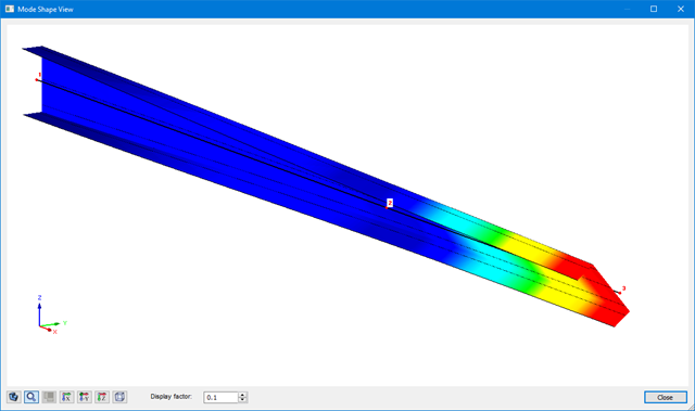
Wyniki analizy skręcania skrępowanego są wyświetlane w modułach RF-/STEEL AISC i RF-/STEEL EC3 w zwykły sposób. Odpowiednie okna wyników zawierają między innymi wartości krytycznego skręcania i skręcania, siły wewnętrzne oraz podsumowanie obliczeń.
Graficzne przedstawienie postaci drgań (wraz z deplanacją) umożliwia realistyczną ocenę zachowania się wyboczenia.