35 Wyniki
Wyświetl wyniki:
Sortuj według:

Tabela wyników modelu budynku 'Wyniki według kondygnacji' przedstawia środek ciężkości przypadków obciążeń i kombinacji obciążeń. Oprócz obciążenia stałego uwzględniane są również obciążenia pionowe odpowiednich przypadków obciążeń i kombinacji obciążeń.
W celu wyświetlenia środka ciężkości z uwzględnieniem wybranego obciążenia można również użyć okna dialogowego 'Środek ciężkości oraz Informacje o wybranych obiektach.

W rozszerzeniu Model budynku można zdefiniować właściwości ścian usztywniających i belek-ścian dla odpowiednich rozszerzeń.

Do modelowania kondygnacji, w przypadku płyt można wykorzystać opcję "Tarcza podatna".
Zasadniczo ta opcja modelowania wybiera to samo podejście, co w przypadku modelowania kondygnacji typu "Sztywna przepona". W przeciwieństwie do sztywnej przepony, sprzężenie węzłowe nie jest przeprowadzane od środka ciężkości do każdego węzła ES. W ten sposób możliwe jest uwzględnienie elastyczności płyty.

- 002842
- Ogólne informacje
- Analiza naprężeniowo-odkształceniowa RFEM 6
- Analiza naprężeniowo-odkształceniowa RSTAB 9
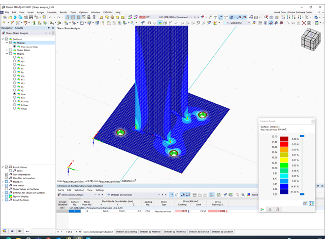
W rozszerzeniu Analiza naprężeniowo-odkształceniowa można użyć opcji, aby określić zależne od znaku naprężenia graniczne za pomocą składowej naprężenia.

- 002829
- Ogólne informacje
- Analiza naprężeniowo-odkształceniowa RFEM 6
- Analiza naprężeniowo-odkształceniowa RSTAB 9
W rozszerzeniu Analiza naprężeniowo-odkształceniowa można zdefiniować cykl naprężeń granicznych zależny od elementu i uwzględnić go w obliczeniach.

Podczas generowania ścian usztywniających i belek-ścian można przydzielać nie tylko powierzchnie i komórki, ale także pręty.

W obliczeniach modelu budynku można pominąć otwory o określonej powierzchni. Funkcję tę można aktywować w ustawieniach globalnych kondygnacji budynku. Pojawi się komunikat ostrzegający, że otwory zostały pominięte.
Model budynku jest obliczany w dwóch etapach:
- Globale 3D-Berechnung des Gesamtmodells, in welchem die Decken als starre Ebene (Diaphragma) oder als Biegeplatte modelliert werden
- Lokale 2D-Berechnung der einzelnen Geschossdecken
Die Ergebnisse der Stützen und Wände aus der 3D-Berechnung und die Ergebnisse der Decken aus der 2D-Berechnung werden nach der Berechnung in einem einzigen Modell zusammengefasst. Dadurch muss zwischen dem 3D-Modell und der einzelnen 2D-Modellen der Decken nicht gewechselt werden. Der Anwender arbeitet nur mit einem Model, spart wertvolle Zeit und vermeidet eventuelle Fehler beim händischen Datenaustausch zwischen dem 3D-Modell und der einzelnen 2D-Decken-Modelle.
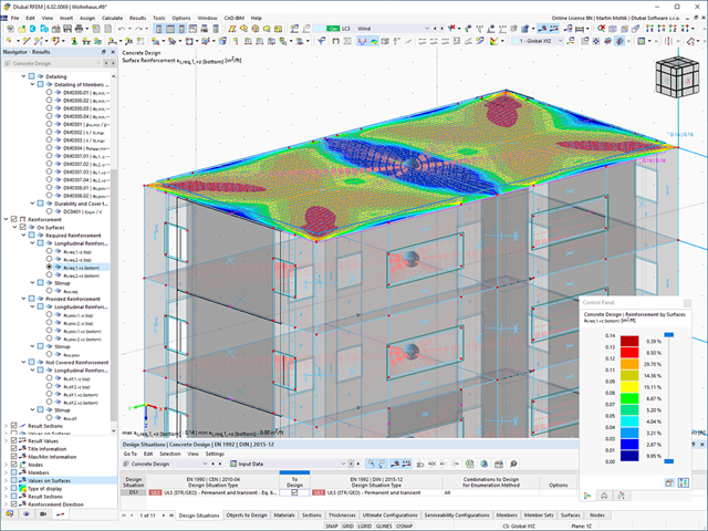
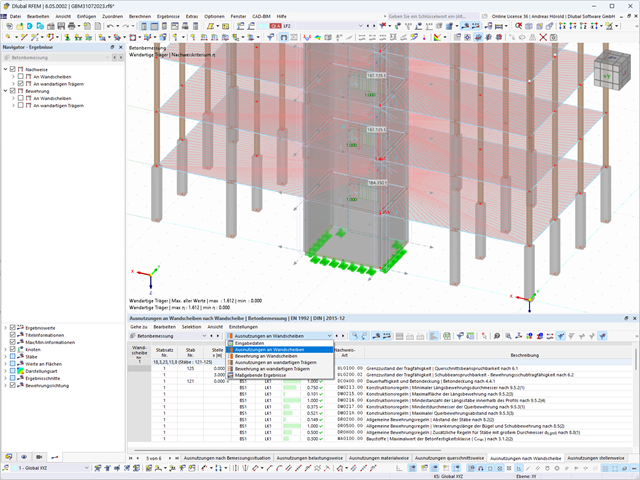
Die vertikalen Flächen im Modell können vom Nutzer in Schubwände (Shear Walls) und Öffnungsstürze (Sprandels) geteilt werden. Aus diesen Wandobjekten erzeugt das Programm automatisch interne Ergebnisstäbe, so dass diese dann nach der gewünschten Norm im Add-On Betonbemessung für RFEM 6 als Stäbe bemessen werden können.
Ściany usztywniające i belki-ściany z modelu budynku są dostępne jako niezależne obiekty w rozszerzeniach. W ten sposób możliwe jest szybsze filtrowanie obiektów w wynikach oraz tworzenie lepszej dokumentacji w raporcie.
Za pomocą generatora kondygnacji w rozszerzeniu Model budynku można automatycznie tworzyć kondygnacje budynku w zależności od topologii modelu.

W przypadku analizy spektrum odpowiedzi modeli budynków można wyświetlić współczynniki wrażliwości dla kierunków poziomych według kondygnacji.
Dzięki tym kluczowym wartościom można zinterpretować wrażliwość na efekty stateczności.
.png?mw=640&hash=403c565ab80c4dd45c2d1356634fb74a90428b70)
W bibliotece konstrukcji warstwowych dostępni są następujący producenci drewna klejonego krzyżowo:
- Binderholz (USA)
- KLH (USA, CAN)
- Kalesnikoff (USA, CAN)
- Nordic Structures (USA, CAN)
- Mercer Mass Timber
- SmartLam
- Sterling Structural
- Konstrukcje nośne wymienione w Lignatec wydanie 32 "Drewno klejone krzyżowo z produkcji szwajcarskiej"
Wczytanie konstrukcji z biblioteki konstrukcji warstw powoduje automatyczne przejęcie wszystkich istotnych parametrów. Biblioteka jest stale aktualizowana.
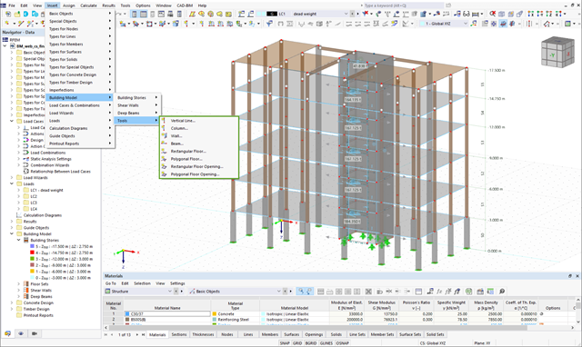
W przypadku elementów w modelach budynków dostępnych jest kilka narzędzi do modelowania:
- Linia pionowa
- Słup
- Ściana
- Belka
- Strop prostokątny
- Płyta wielokątna
- Prostokątny otwór w stropie
- Wielokątny otwór w stropie
Ta funkcja umożliwia definicję elementów na płaszczyźnie podłoża (na przykład z warstwą tła) z powiązanym tworzeniem wielu elementów w przestrzeni.
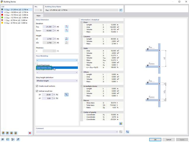
Korzystając z kondygnacji typu "Tylko przenoszenie obciążenia", można uwzględnić w rozszerzeniu Model budynku stropy bez wpływu sztywności do i z płaszczyzny. Ten typ elementu zbiera obciążenia na stropie i przenosi je na elementy nośne modelu 3D. Daje to możliwość symulacji w modelu 3D elementów drugorzędnych, takich jak np. ruszt i inne podobne elementy rozkładu obciążenia, bez dalszych efektów.
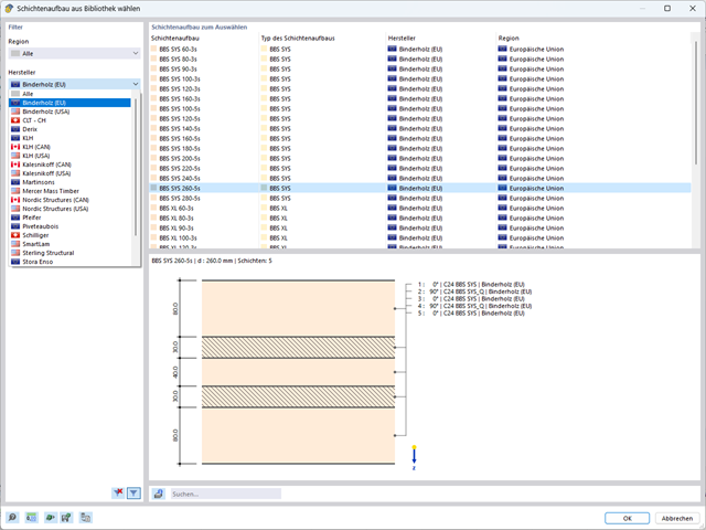
W programie RFEM zaimplementowano bibliotekę płyt z drewna klejonego krzyżowo, z której można importować konstrukcje warstwowe różnych producentów (np. Binderholz, KLH, Piveteaubois, Södra, Züblin Timber, Schilliger, Stora Enso). Oprócz grubości i materiałów warstw podane są również informacje o redukcji sztywności i łączeniu wąskich boków.
Przejdź do filmu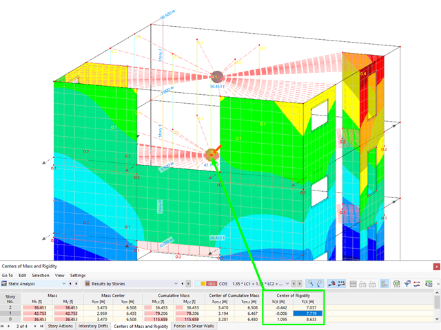
Aktywowałeś rozszerzenie Model budynku ? Bardzo dobrze! Możesz wyświetlić środek sztywności w tabeli i w formie graficznej. Użyj go na przykład do analizy dynamicznej.
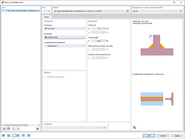
W programie RFEM 6 możliwe jest definiowanie spoin liniowych między powierzchniami i obliczanie naprężeń w spoinie za pomocą rozszerzenia Analiza naprężeniowo-odkształceniowa.
Dostępne są następujące typy połączeń:
- połączenie stykowe
- Złącze narożne
- Złącze zakładkowe
- Złącze teowe
W zależności od typu połączenia dostępne są następujące typy spoin:
- Pojedynczy kwadrat
- Podwójny
- Podwójny ukos
- Spoina typu V
- Spoina typu 2 V
- Spoina typu U
- Spoina typu 2 U
- Spoina typu J
- Spoina typu 2 J
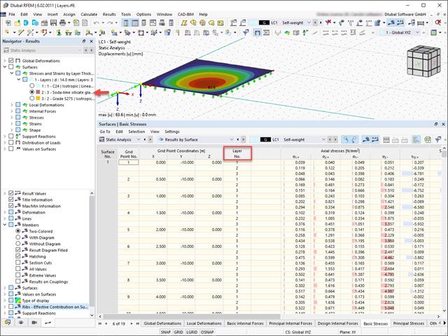
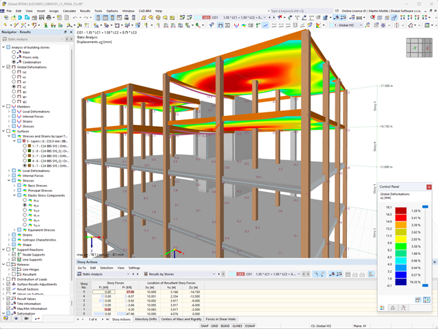
Wyniki naprężeń i odkształceń według powierzchni można wyświetlić w tabeli wyników powierzchni zgodnie z grubością warstwy.
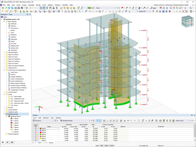
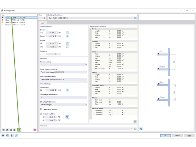
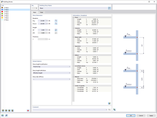
Obawiasz się, że Twój projekt skończy się cyfrową wieżą Babel? Rozszerzenie Model budynku dla RFEM wspomaga pracę nad wielokondygnacyjnym projektem budowlanym. Tutaj możesz definiować i manipulować budynkiem za pomocą kondygnacji. Kondygnacje można później dostosować na wiele sposobów, a także wybrać sztywność płyty. Informacje na temat kondygnacji i całego modelu (środek ciężkości, środek sztywności) są wyświetlane w tabelach i na grafice.

- 002232
- Ogólne informacje
- Optymalizacja i koszty | Szacowanie emisji CO2 RFEM 6
- Optymalizacja i koszty | Szacowanie emisji CO2 RSTAB 9
Możesz być pewien, że koszty są ważnym czynnikiem w planowaniu konstrukcyjnym każdego projektu. Należy również przestrzegać przepisów dotyczących szacowania emisji. Dwuczęściowe rozszerzenie Optymalizacja i koszty/Szacowanie emisji CO2 ułatwia odnalezienie się w gąszczu norm i opcji. Wykorzystuje technologię sztucznej inteligencji (AI) optymalizacji rojem cząstek (PSO) w celu znalezienia odpowiednich parametrów dla sparametryzowanych modeli i bloków, które zagwarantują zgodność ze zwykłymi kryteriami optymalizacji. Ponadto, rozszerzenie oszacowuje koszty modelu lub emisję CO2 poprzez określenie kosztów jednostkowych lub emisji jednostkowej dla materiałów zdefiniowanych w modelu konstrukcyjnym. Dzięki temu rozszerzeniu jesteś po bezpiecznej stronie.

Dzięki rozszerzeniu Analiza historii czasowej (TDA) można uwzględnić zmienne w czasie zachowanie materiału w przypadku prętów i powierzchni. Długotrwałe efekty, takie jak pełzanie, skurcz i starzenie, mogą wpływać na rozkład sił wewnętrznych, w zależności od konstrukcji. Darauf bereiten Sie sich mit diesem Add-On optimal vor.
Dla każdego przypadku obciążenia można wyświetlić odkształcenia w czasie końcowym.
Wyniki te są również dokumentowane w protokole wydruku programów RFEM i RSTAB. Zawartość protokołu i jego zakres można wybrać specjalnie dla poszczególnych warunków projektowych.
- 002169
- Ogólne informacje
- Analiza naprężeniowo-odkształceniowa RFEM 6
- Analiza naprężeniowo-odkształceniowa RSTAB 9
W porównaniu z modułem dodatkowym RF-/STEEL (RFEM 5/RSTAB 8) do rozszerzenia Analiza naprężeniowo-odkształceniowa dla programu RFEM 6/RSTAB 9 dodano następujące nowe funkcje:
- Możliwość analizy prętów, powierzchni, brył, spoin (połączenia spawane liniowo między dwiema i trzema powierzchniami z późniejszym obliczaniem naprężeń)
- Wyświetlanie naprężeń, stopni naprężeń, zakresów naprężeń i odkształceń
- Naprężenie graniczne w zależności od przydzielonego materiału lub danych wejściowych zdefiniowanych przez użytkownika
- Indywidualne określenie wyników do obliczeń poprzez dowolnie przydzielane typów ustawień
- Szczegóły dla wyników niemodalnych z wyświetlaniem przygotowanego wzoru i dodatkowym wyświetlaniem wyników na poziomie przekroju prętów
- Możliwość wygenerowania zastosowanych wzorów do kontroli obliczeń

- 002108
- Ogólne informacje
- Optymalizacja i koszty | Szacowanie emisji CO2 RFEM 6
- Optymalizacja i koszty | Szacowanie emisji CO2 RSTAB 9
- Technologia sztucznej inteligencji (AI): Optymalizacja roju cząstek (PSO)
- Optymalizacja konstrukcji ze względu na minimalny ciężar lub deformację
- Możliwość zastosowania dowolnej liczby parametrów optymalizacyjnych
- Określanie zakresów zmiennych
- Optymalizacja przekrojów i materiałów
- Typy definicji parametrów
- Optymalizacja | Rosnąco, czyli optymalizacja | Malejąca
- Zastosowanie parametrycznych modeli i bloków
- Parametryzacja bloków w języku JavaScript na podstawie kodu
- Optymalizacja z uwzględnieniem wyników obliczeń
- Tabelaryczne przedstawienie najlepszych mutacji modelu
- Wyświetlanie w czasie rzeczywistym mutacji modelu w procesie optymalizacji
- Kalkulacja kosztów modelu dzięki zadanym cenom jednostkowym
- Określanie potencjału tworzenia efektu cieplarnianego (GWP-global warming potential) na etapie tworzenia modelu poprzez szacowanie równoważnej emisji CO2
- Określanie jednostkowych wskaźników zależnych od masy, objętości i powierzchni (cena i emisja CO2)

- 002109
- Ogólne informacje
- Optymalizacja i koszty | Szacowanie emisji CO2 RFEM 6
- Optymalizacja i koszty | Szacowanie emisji CO2 RSTAB 9
Masz pytania dotyczące programu? Optymalizacja konstrukcji w programach RFEM i RSTAB jest uzupełnieniem parametrycznego wprowadzania danych. Jest to proces równoległy, niezależny od rzeczywistych obliczeń modelu wraz ze wszystkimi jego zwykłymi definicjami obliczeń i obliczeń. Rozszerzenie zakłada, że model lub blok jest zbudowany w kontekście parametrycznym i jest kontrolowany przez globalne parametry kontrolne typu "optymalizacja". Dlatego te parametry kontrolne mają dolną i górną granicę oraz wielkość kroku w celu ograniczenia zakresu optymalizacji. Aby znaleźć optymalne wartości parametrów kontrolnych, należy określić kryterium optymalizacji (na przykład minimalny ciężar) przy wyborze metody optymalizacji (na przykład optymalizacja roju cząstek).
Oszacowanie kosztów i emisji CO2 można znaleźć już w definicjach materiałów. Obie opcje można aktywować osobno w każdej definicji materiału. Oszacowanie oparte jest na koszcie jednostkowym lub jednostkowej wartości emisji dla prętów, powierzchni oraz brył. W tym przypadku można wybrać, czy jednostki mają zostać podane według masy, objętości czy powierzchni.

- 002110
- Ogólne informacje
- Optymalizacja i koszty | Szacowanie emisji CO2 RFEM 6
- Optymalizacja i koszty | Szacowanie emisji CO2 RSTAB 9
Istnieją dwie metody optymalizacji, dzięki którym można znaleźć optymalne wartości parametrów według kryterium ciężaru lub odkształcenia.
Najbardziej wydajną metodą o najkrótszym czasie obliczeń jest optymalizacja roju cząstek zbliżona do naturalnej (PSO). Czy słyszałeś lub czytałeś o tym? Ta technologia sztucznej inteligencji (AI) ma silną analogię do zachowania stad zwierząt szukających miejsca odpoczynku. W takich rojach można znaleźć wiele osób (por. rozwiązanie optymalizacyjne - na przykład waga), które lubią przebywać w grupie i podążać za ruchem grupy. Załóżmy, że każdy pręt roju musi zostać poddany spoczynkowi w optymalnym miejscu (por. najlepsze rozwiązanie - na przykład najniższa waga). Potrzeba ta wzrasta wraz ze zbliżaniem się do miejsca odpoczynku. Na zachowanie roju mają zatem wpływ również właściwości przestrzeni (por. wykres wyników).
Dlaczego wycieczka do biologii? Po prostu - proces PSO w RFEM lub RSTAB przebiega w podobny sposób. Proces obliczeń rozpoczyna się od wyniku optymalizacji poprzez losowe przypisanie parametrów, które mają zostać zoptymalizowane. Wielokrotnie określa nowe wyniki optymalizacji ze zróżnicowanymi wartościami parametrów, które opierają się na doświadczeniach z wcześniej przeprowadzonych mutacji modelu. Proces jest kontynuowany do momentu osiągnięcia określonej liczby możliwych mutacji modelu.
Jako alternatywa dla tej metody program oferuje również metodę przetwarzania wsadowego. Metoda ta ma na celu sprawdzenie wszystkich możliwych mutacji modelu poprzez losowe określanie wartości parametrów optymalizacji, aż do osiągnięcia określonej liczby możliwych mutacji modelu.
Po obliczeniu mutacji modelu obydwa warianty sprawdzają również odpowiednie aktywowane wyniki obliczeń rozszerzeń. Ponadto zapisuje on wariant z odpowiednim wynikiem optymalizacji i przypisaniem wartości parametrów optymalizacji, jeżeli wykorzystanie jest < 1.
Na podstawie odpowiednich sum poszczególnych materiałów można określić szacunkowe koszty całkowite i emisję. Na sumę materiałów składają się zależne od ciężaru, objętości i powierzchnie elementów prętowych, powierzchniowych i bryłowych.

- 002161
- Ogólne informacje
- Optymalizacja i koszty | Szacowanie emisji CO2 RFEM 6
- Optymalizacja i koszty | Szacowanie emisji CO2 RSTAB 9
Obie metody optymalizacji mają jedną wspólną cechę. Na końcu procesu wyświetlają listę wariacji modelu na podstawie przechowywanych danych. Można tu znaleźć szczegóły na temat wyniku decydującego dla optymalizacji i odpowiadające mu wartości parametrów. Lista jest zorganizowana w porządku malejącym. Zakładane najlepsze rozwiązanie znajduje się na górze. W takim przypadku wynik optymalizacji wraz z wyznaczoną wartością jest najbardziej zbliżony do kryterium optymalizacji. Wszystkie dodatkowe wyniki pokazują wykorzystanie < 1. Ponadto, po zakończeniu analizy, program dostosuje wartości na globalnej liście parametrów, aby odpowiadały tym dla optymalnego rozwiązania.
W oknach dialogowych materiałów znajdują się dodatkowe zakładki "Oszacowanie kosztów" i "Oszacowanie emisji CO2". Tutaj wyświetlane są indywidualne szacunkowe sumy przydzielonych prętów, powierzchni i objętości na jednostkę masy, objętości i powierzchni. Dodatkowo zakładki te podają całkowity koszt i emisję wszystkich przydzielonych do konstrukcji materiałów. Zapewnia to dobry przegląd projektu.
_ENG.png?mw=640&hash=1053c9bef400e9f5361c9c3278f76a272fcc4ddf)
Czy aktywowałeś rozszerzenie Analiza historii czasowej (TDA)? Dobrze, teraz można dodawać dane czasowe do przypadków obciążeń. Po zdefiniowaniu początku i końca obciążenia, uwzględniany jest wpływ pełzania na końcu obciążenia. Program umożliwia modelowanie efektów pełzania w konstrukcjach szkieletowych i kratowych wykonanych z betonu zbrojonego.
W tym przypadku obliczenia są przeprowadzane nieliniowo zgodnie z modelem reologicznym (model Kelvina i Maxwella).
Czy obliczenia zakończyły się pomyślnie? Wyznaczone siły wewnętrzne można teraz wyświetlić w tabelach i grafice, a także uwzględnić w obliczeniach.
- Uwzględnianie i wyświetlanie mas kondygnacji
- Lista elementów konstrukcyjnych i ich informacje
- Automatyczne tworzenie przekrojów wynikowych na ścianach usztywniających
- Wyświetlanie wypadkowych przekrojów w kierunku globalnym do wyznaczania sił tnących
- Opcjonalna definicja sztywnej membrany według kondygnacji (modelowanie kondygnacji)
- Typ sztywności Płyta stropowa - tarcza sztywna
- Definiowanie zbiorów stropów,
- na przykład obliczanie płyt jako pozycji 2D w modelu 3D
- Ściany usztywniające: Automatyczne definiowanie prętów wynikowych o dowolnym przekroju
- Wymiarowanie przekrojów prostokątnych z wykorzystaniem rozszerzenia Projektowanie konstrukcji betonowych
- Definicja belek-ścian
- Wymiarowanie możliwe dzięki rozszerzeniu Projektowanie konstrukcji betonowych
- Tabelaryczne przedstawianie oddziaływań kondygnacji, znoszenia międzykondygnacyjnego oraz punktów środkowych masy i sztywności, jak również sił w ścianach usztywniających
- Oddzielne wyświetlanie wyników dla obliczeń stropu i usztywnień
- Opcjonalne pominięcie otworów o określonym rozmiarze
W przypadku modelu budynku dostępne są dwie opcje. Można go utworzyć na początku modelowania konstrukcji lub aktywować później. W modelu budynku można bezpośrednio definiować kondygnacje i modyfikować je.
Podczas manipulowania kondygnacjami można wybrać, czy zostaną zmodyfikowane, czy zachowane, korzystając z różnych opcji.
Program RFEM wykonuje część pracy za Ciebie. Na przykład, program automatycznie generuje przekroje wynikowe,'dzięki czemu nie trzeba wykonywać wielu obliczeń.