12 Wyniki
Wyświetl wyniki:
Sortuj według:
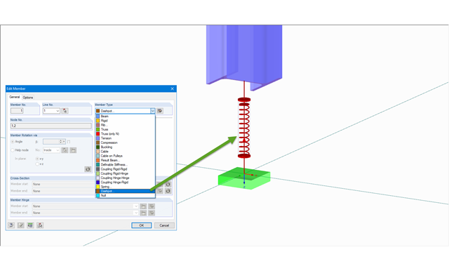
Typ pręta 'Dashpot' może być wykorzystywany do analizy przebiegu czasowego w RFEM/RSTAB z modułami dodatkowymi RF-/DYNAM Pro - Forced Vibrations i RF-/DYNAM Pro - Nonlinear Time History. Ten liniowy lepki element tłumiący uwzględnia siły w zależności od prędkości.
Pod względem lepkosprężystości typ pręta 'Dashpot' jest podobny do modelu Kelvina-Voigta, który składa się z elementu tłumiącego i sprężyny (oba elementy połączone równolegle).
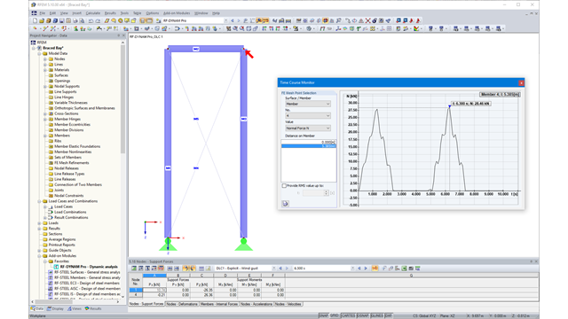
Dzięki integracji RF-/DYNAM Pro z programem RFEM lub RSTAB, do globalnego raportu można włączać numeryczne i graficzne wyniki z RF-/DYNAM Pro - Nonlinear Time History. Ponadto wszystkie opcje w programach RFEM i RSTAB są dostępne do wizualizacji graficznej. Wyniki analizy przebiegu czasowego wyświetlane są na wykresie przebiegu czasowego.
Wyniki są wyświetlane w funkcji czasu, a wartości liczbowe można eksportować do programu MS Excel. Kombinacje wyników mogą być eksportowane jako wynik pojedynczego kroku czasowego lub najbardziej niekorzystne wyniki wszystkich kroków czasowych są odfiltrowywane.
Obliczenia w RFEM
Nieliniowa analiza przebiegu czasowego jest przeprowadzana za pomocą pośredniej analizy Newmarka lub analizy bezpośredniej. Obie metody są metodami bezpośredniej integracji czasu. Analiza pośrednia wymaga definiowania małych kroków czasowych w celu dostarczenia dokładnych wyników. Analiza bezpośrednia określa automatycznie wymagany krok czasowy, w celu zapewnienia stabilności rozwiązania. Analizę bezpośrednią stosuje się w przypadku obliczania krótkotrwałych wzbudzeń, takich jak wzbudzenia impulsowe lub wybuch.
Obliczenia w RSTAB
Nieliniowa analiza przebiegu czasowego jest przeprowadzana z wykorzystaniem analizy bezpośredniej. Jest to metoda bezpośredniej integracji czasu i określa automatycznie krok czasowy, konieczny w celu zapewnienia stabilności wyników obliczeń.

- 001351
- Moduły dodatkowe
- RF-Dynam Pro (en) | Nieliniowa historia czasowa 5
- Analiza dynamiczna i sejsmiczna
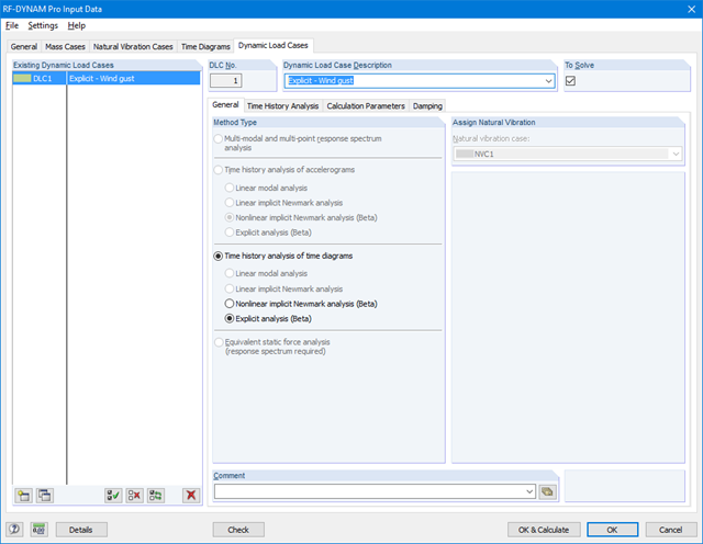
RF-/DYNAM Pro - Nonlinear Time History jest zintegrowany z RF‑/DYNAM Pro - Forced Vibrations i rozszerzony o dwie metody analizy nieliniowej (jedna analiza nieliniowa w RSTAB).
Wykresy siła-czas mogą być wprowadzane jako przejściowe, okresowe lub jako funkcje czasu. Dynamiczne przypadki obciążeń stanowią połączenie wykresów czasowych ze statycznymi przypadkami obciążeń, co zapewnia dużą elastyczność. Ponadto, istnieje możliwość definiowania kroków czasowych do obliczeń, tłumienia konstrukcji i opcji eksportu w dynamicznych przypadkach obciążeń.

- 001349
- Ogólne informacje
- RF-Dynam Pro (en) | Nieliniowa historia czasowa 5
- Analiza dynamiczna i sejsmiczna
- Nieliniowe typy prętów, takie jak pręty ściskane i rozciągane lub kable
- Nieliniowości pręta, takie jak uszkodzenie, przerwanie, uplastycznienie pod wpływem rozciągania lub ściskania
- Nieliniowości podpory, takie jak uszkodzenie, tarcie, wykres i częściowa aktywność
- Nieliniowości zwolnienia, takie jak tarcie, częściowa aktywność, wykres oraz uszkodzenie w przypadku, gdy siły wewnętrzne są dodatnie lub ujemne
.png?mw=640&hash=8cfd0c4bd093c03de543d147ffbf6f5c9250634a)
- 001348
- Ogólne informacje
- RF-Dynam Pro (en) | Nieliniowa historia czasowa 5
- Analiza dynamiczna i sejsmiczna
- Zdefiniowane przez użytkownika wykresy czasowe w funkcji czasu, w formie tabelarycznej lub jako obciążenia harmoniczne
- Połączenie wykresów czasowych z przypadkami lub kombinacjami obciążeń w programie RFEM/RSTAB (definiowanie obciążeń węzłowych, prętowych i powierzchniowych oraz zmiennych w czasie obciążeń wolnych i obciążeń)
- Możliwość połączenia kilku niezależnych oddziaływań wzbudzonych
- Nieliniowa analiza przebiegu czasowego z niejawną analizą Newmarka (tylko w RFEM) lub analizą bezpośrednią
- Tłumienie konstrukcji przy użyciu współczynnika Rayleigha lub tłumienia Lehra's
- Bezpośredni import początkowych deformacji z przypadku obciążenia lub kombinacji obciążeń (tylko RFEM)
- Modyfikacje sztywności jako warunki początkowe; na przykład wpływ siły osiowej, dezaktywowane pręty (tylko RSTAB)
- Graficzne przedstawienie rezultatów na diagramie przebiegu czasowego
- Eksport wyników w zdefiniownych przez użytkownika krokach czasowych lub jako obwiednia
Dane dotyczące materiału, obciążeń i kombinacji obciążeń muszą zostać wprowadzone w programie RFEM/RSTAB zgodnie z założeniami obliczeniowymi określonymi w Code of Practice for the Structural Use of Steel 2011 (Buildings Department – Hong Kong).
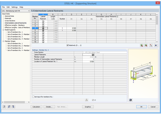
W module RF-/STEEL HK wybiera się najpierw pręty i zbiory prętów, które mają zostać obliczone, a następnie przypadki, grupy i kombinacje obciążeń. W kolejnych oknach wprowadzania można dostosować wstępnie zdefiniowane ustawienia bocznych podpór pośrednich i długości efektywnych.
W przypadku prętów ciągłych można zdefiniować indywidualne warunki podparcia i mimośrody każdego węzła pośredniego pojedynczych prętów. Specjalne narzędzie MES określa następnie obciążenia krytyczne i momenty wymagane do analizy stateczności w takich sytuacjach.
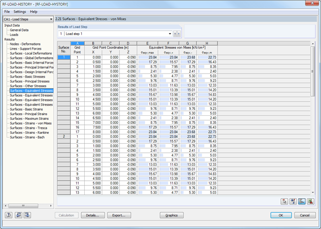
Po zakończeniu obliczeń wyniki poszczególnych kroków obciążenia można ocenić bezpośrednio w oknach modułu lub graficznie w modelu konstrukcyjnym.
Wyniki obejmują na przykład odkształcenia, naprężenia i siły wewnętrzne powierzchni oraz odkształcenia i naprężenia brył. Kombinacje wyników dla każdego kroku obciążenia można eksportować do programu RFEM. Kombinacje obwiedni można wykorzystać do dalszych obliczeń w innych modułach dodatkowych dla programu RFEM.
Wszystkie dane wejściowe i wyniki modułu dodatkowego stanowią część globalnego protokołu wydruku programu RFEM.
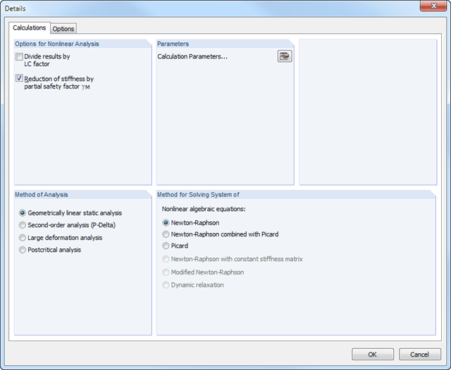
Obliczenia są przeprowadzane sukcesywnie dla każdego kroku obciążenia. Odkształcenia stałe (plastyczne) poprzednich kroków obciążenia są uwzględniane przy obliczaniu dalszych kroków obciążenia. W ten sposób możliwe jest również przeprowadzenie obliczeń z uwzględnieniem podparcia konstrukcji.
Obciążenia poszczególnych kroków są sumowane (w zależności od znaków) w trakcie całego procesu obliczeniowego. Można wybrać dowolną metodę analizy (liniowa, statyczna, analiza dużych deformacji i analiza postkrytyczna). Ponadto moduł zarządza globalnymi ustawieniami obliczeń.
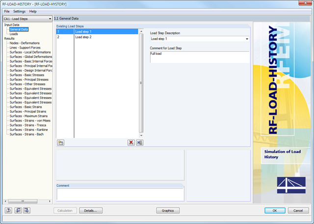
Po zdefiniowaniu całego modelu i obciążenia w programie RFEM, w oknie 1.1 Dane ogólne można wprowadzić kroki i opisy obciążeń.
W oknie 1.2 Obciążenia można przydzielić przypadki obciążeń lub kombinacje obciążeń do różnych przyrostów obciążenia. Można je pomnożyć przez współczynnik obciążenia.
.png?mw=640&hash=31ebb9c47d4f8334d4a27ff248233fc0442a2e72)
- Proste definiowanie przyrostów obciążenia
- Łatwe przypisywanie przypadków obciążeń i kombinacji obciążeń do przyrostów obciążeń
- Uwzględnienie odkształceń plastycznych (hartowanie izotropowe) poprzednich przyrostów obciążenia
- Wyniki (odkształcenia, siły podporowe, siły wewnętrzne, naprężenia, odkształcenia itp.) są wyświetlane numerycznie i graficznie dla poszczególnych przyrostów obciążenia
- Szczegółowy protokół wydruku zawierający dokumentację wyników dla wszystkich przyrostów obciążenia
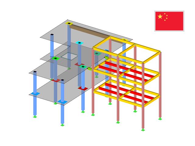
Dodatkowo dostępne są obliczenia sejsmiczne według normy GB 50011-2010 (Code for seismic design of buildings). Biblioteka materiałów zawiera chińskie rodzaje betoów oraz stali zbrojeniowej.
Ponadto zawsze możliwe jest określanie własnych materiałów zgodnie z normą GB 50010.