15736x

001525

Dipl.-Ing. (FH) Bastian Kuhn, M.Sc.

2018-06-27

Orthotropic Material Laws

Orthotropic material laws are used wherever materials are arranged according to their loading. Examples include fiber-reinforced plastics, trapezoidal sheets, reinforced concrete, and timber.

As a rule, the Hooke's material law

ν = \frac{E}{2 G} - 1 \leq 0.5

Formula 1

and

- 1 < ν < 0.5

Formula 2

is no longer valid for orthotropic materials.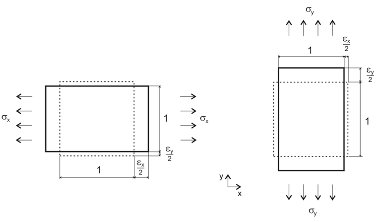

Transverse Strain

The following material parameters refer to two-dimensional stiffnesses and, unless otherwise stated, to the material of timber. A local axis system is the basis, as shown in Image 01.

E_x = stiffness in the local x-direction of the surface
E_y = the stiffness in the local y-direction of the surface
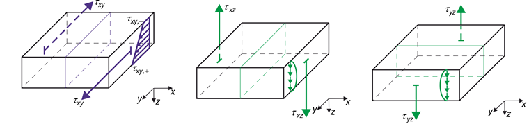
G_xz = the shear stiffness in the local x-direction of the surface (thickness direction of the plate)
G_yz = the shear stiffness in the local y-direction of the surface (thickness direction of the plate)
G_xy = the in-plane shear stiffness
ν_xy = the transversal strain in the x-direction
ν_yx = the transversal strain in the y-direction

The stresses in Image 02 are related to the stiffnesses mentioned here.

Shear Stresses

The material law is subject to the following rules.

Equation 1:

\frac{ν_{yx}}{E_{y}} = \frac{ν_{xy}}{E_{x}}

Formula 3

Equation 2:

ν_{xy} ⩾ ν_{yx}

Formula 4

Equation 3:

ν_{xy} = - \frac{ε_{y}}{ε_{x}} = \frac{E_{x}}{E_{y}} \cdot ν_{yx}

Formula 5

Equation 4 (in-plane stiffnesses):

[\begin{matrix} ε_{x} \\ ε_{y} \\ γ_{xy} \end{matrix}] = [\begin{matrix} \frac{1}{E_{x}} & - \frac{ν_{xy}}{E_{x}} & 0 \\ - \frac{ν_{xy}}{E_{x}} & \frac{1}{E_{y}} & 0 \\ 0 & 0 & G_{xy} \end{matrix}] \cdot [\begin{matrix} σ_{x} \\ σ_{y} \\ τ_{xy} \end{matrix}]

Formula 6

The ratio of the strains in the equations mentioned above underlines the relations in Image 01.

The in-plane stiffnesses are calculated as follows.

Equation 5:

d_{i} = [\begin{matrix} d_{11, i} & d_{12, i} & 0 \\ d_{22, i} & 0 \\ sym & d_{33, i} \end{matrix}] = [\begin{matrix} \frac{E_{x, i}}{1 - ν_{xy, i}^{2} \frac{E_{y, i}}{E_{x, i}}} & \frac{ν_{xy, i} E_{y, i}}{1 - ν_{xy, i}^{2} \frac{E_{y, i}}{E_{x, i}}} & 0 \\ \frac{E_{y, i}}{1 - ν_{xy, i}^{2} \frac{E_{y, i}}{E_{x, i}}} & 0 \\ sym & G_{xy, i} \end{matrix}]

Formula 7

Transversal Strain ν

As already explained in Image 01, the smoother material behavior in the respective direction results in altered deformations and stresses in this direction.

Ratio of the strains:

Equation 6:

ν_{xy} = - \frac{ε_{y}}{ε_{x}} \to ε_{y} = - ν_{x} \cdot ε_{x}

Formula 8

Equation 7:

ν_{yx} = - \frac{ε_{x}}{ε_{y}} \to ε_{x} = - ν_{y} \cdot ε_{y}

Formula 9

For

σ_{x} \neq 0, σ_{y} = 0, σ_{xy} = 0

Formula 10

the following equations result with Hooke's law.

Equation 8:

ε_{x} = \frac{σ_{x}}{E_{x}}

Formula 11

Equation 9:

ε_{y} = \frac{σ_{y}}{E_{y}}

Formula 12

Equation 10:

σ_{y} = ε_{y} \cdot E_{y} with E_{y} = \frac{ν_{yx} \cdot E_{x}}{ν_{xy}} \to σ_{y} = ε_{y} \cdot \frac{ν_{yx} \cdot E_{x}}{ν_{xy}}

Formula 13

Equation 11:

\to σ_{y} = ε_{y} \cdot \frac{ν_{yx} \cdot \frac{σ_{x}}{ε_{x}}}{ν_{xy}}

Formula 14

Equation 12:

\to ε_{y} = \frac{ε_{y} \cdot \frac{ν_{yx} \cdot \frac{σ_{x}}{ε_{x}}}{ν_{xy}}}{E_{y}} with ν_{xy} = - \frac{ε_{y}}{ε_{x}}

Formula 15

Equation 13:

\to ε_{y} = \frac{ε_{y} \cdot ν_{yx} \cdot σ_{x}}{ε_{x} \cdot (- \frac{ε_{y}}{ε_{x}}) \cdot E_{y}} = - \frac{ν_{yx} \cdot σ_{x}}{E_{y}}

Formula 16

Stiffness Matrix

Caculation of the global stiffness matrix of the plate.

Equation 14:

D = [\begin{matrix} D_{11} & D_{12} & 0 & 0 & 0 & 0 & 0 & 0 \\ D_{22} & 0 & 0 & 0 & 0 & 0 & 0 \\ D_{33} & 0 & 0 & 0 & 0 & 0 \\ D_{44} & 0 & 0 & 0 & 0 \\ D_{55} & 0 & 0 & 0 \\ sym & D_{66} & 0 & 0 \\ D_{77} & 0 \\ D_{88} \end{matrix}]

Formula 17

Bending Components:

Equation 15:

D_{11} = \frac{d^{3}}{12} \cdot d_{11} \hat{=} \frac{E_{x} d^{3}}{12 (1 - ν_{xy} ν_{yx})}

Formula 18

Equation 16:

D_{12} = \frac{d^{3}}{12} \cdot d_{12} \hat{=} sgn (ν_{xy}) \sqrt{ν_{xy} ν_{yx} D_{11} D_{22}}

Formula 19

Equation 17:

D_{22} = \frac{d^{3}}{12} \cdot d_{22} \hat{=} \frac{E_{y} d^{3}}{12 (1 - ν_{xy} ν_{yx})}

Formula 20

Equation 18:

D_{33} = \frac{d^{3}}{12} \cdot d_{33} \hat{=} G_{xy} \frac{d^{3}}{12}

Formula 21

Membrane Components:

Equation 19:

D_{66} = d \cdot d_{11} \hat{=} \frac{E_{x} d}{1 - ν_{xy} ν_{yx}}

Formula 22

Equation 20:

D_{67} = d \cdot d_{12} \hat{=} sgn (ν_{xy}) \sqrt{ν_{xy} ν_{yx} D_{66} D_{77}}

Formula 23

Equation 21:

D_{77} = d \cdot d_{22} \hat{=} \frac{E_{y} d}{1 - ν_{xy} ν_{yx}}

Formula 24

Equation 22:

D_{88} = d \cdot d_{33} \hat{=} G_{xy} d

Formula 25

Shear Components:

Equation 23:

D_{44} = \frac{5}{6} G_{xz} \cdot d

Formula 26

Equation 24:

D_{55} = \frac{5}{6} G_{yz} \cdot d

Formula 27

A prerequisite for these equations is that the stiffness matrix is defined positive, so that all eigenvalues of the matrix are positive.

For this reason, RFEM checks, among other things, the definition of the transversal strain according to the following equation.

Equation 25:

ν_{xy} \leq 0.999 \cdot \sqrt{\frac{E_{x}}{E_{y}}}

Formula 28

Example

The orthotropic material behavior will be explained with the following example (Image 03). An orthotropic material will be compared to an isotropic material. In addition, the stiffness of the orthotropic plate will be defined with the high stiffness in the x-direction and in the y-direction.

System

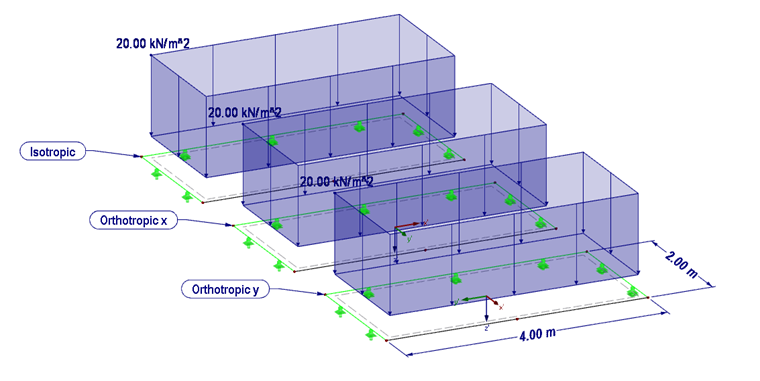
Structure:

Plate thickness 200 mm
Material C 24
Orthotropic stiffnesses

$\begin{array}{l} E_{x} = 1, 100.0 kN / {cm}^{2} \\ E_{y} = 37.0 kN / {cm}^{2} \\ G_{y} = 6.9 kN / {cm}^{2} \\ G_{x} = 69.0 kN / {cm}^{2} \\ G_{xy} = 69.0 kN / {cm}^{2} \\ ν_{xy} = 2.52 \\ ν_{yx} = 0.085 \end{array}$

Formula 29
Isotropic stiffnesses

$\begin{array}{l} E = 1, 100 kN / {cm}^{2} \\ G = 500 kN / {cm}^{2} \\ ν = 0.1 \end{array}$

Formula 30
Dimension w = 2.0 m, l = 4.0 m
Load 20 kN/m²
FE mesh size 50 cm

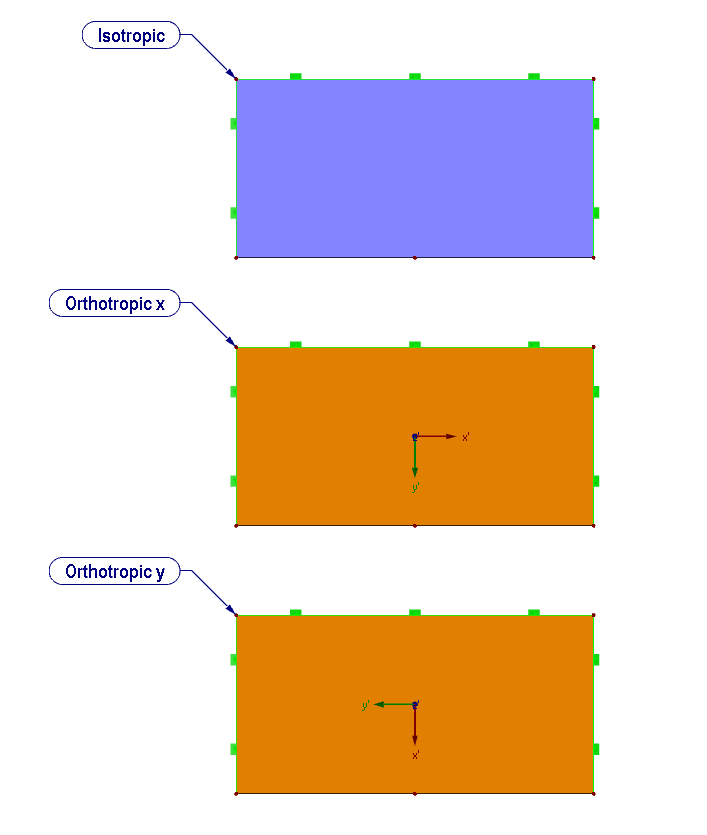
The structure is supported as rigidly fixed in the vertical z-direction. The support conditions in the x- and y-directions have been selected in such a way that no effects occur due to restraint.

The calculation is performed according to the linear static analysis with linear elastic material behavior and support conditions.

The following transversal strain results from Hooke's law, together with the given values.

Equation 26:

ν = (\sqrt{E_{x} \cdot E_{y}}) / (2 G) - 1 = 6.97

Formula 31

This high transversal strain is impossible with the selected material model. With the equations from [1], the values can, however, be adjusted.

Equation 27:

ν_{xy} \approx (\frac{\sqrt{E_{x} E_{y}}}{2 G_{xy}} - 1) \cdot \sqrt{\frac{E_{x}}{E_{y}}}

Formula 32

Equation 28:

ν_{yx} \approx (\frac{\sqrt{E_{x} E_{y}}}{2 G_{xy}} - 1) \cdot \sqrt{\frac{E_{y}}{E_{x}}}

Formula 33

Equation 29:

ν_{xy} = (\frac{\sqrt{1, 100 \cdot 37}}{2 \cdot 69} - 1) \sqrt{\frac{1, 100}{37}} = 2.52

Formula 34

Equation 30:

ν_{xy} = (\frac{\sqrt{1, 100 \cdot 37}}{2 \cdot 69} - 1) \sqrt{\frac{37}{1, 100}} = 0.085

Formula 35

Surfaces with Stiffnesses

Results:
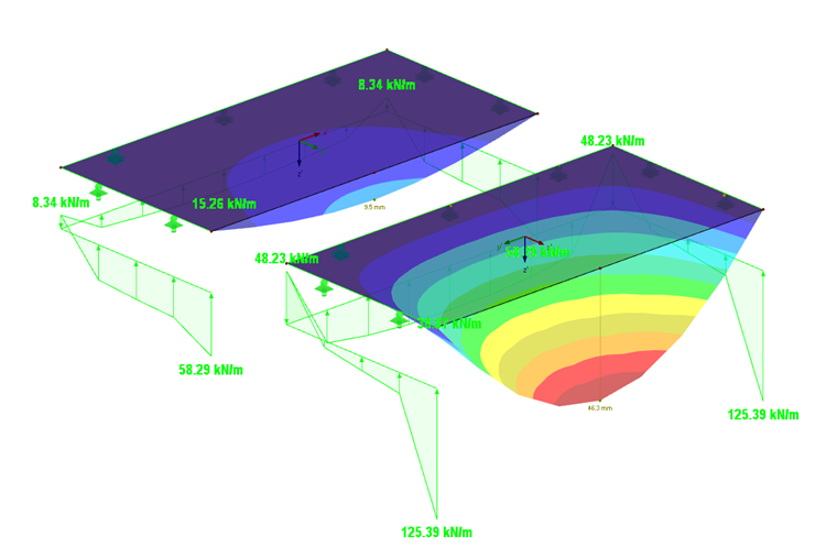
As expected, the largest deformations occur with the orientation of the stiffnesses in the y-direction (Image 06). The support reaction and the moment of the isotropic plate are displayed in Image 05.

Isotropic Material Results

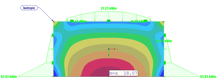
Since the plate with high stiffness in the y-direction (E_y = 1,100 kN/cm²) has high resistance in this direction, the support reactions are also higher there (125.4 kNm compared to 58.3 kNm).

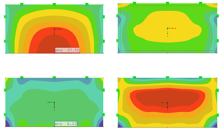
Deformations and Support Reactions of Orthotropic Plates

The resulting maximum bending moments for the orthotropic plates are equal to m_x with the stiffness in the x-direction and for m_y with a high stiffness in the y-direction.

For the plate with high stiffness in the y-direction, the maximum bending moment m_yis almost in the center of the plate (Image 07).

Bending Moments of Orthotropic Plate mx (Left) and my (Right)

Variation of Transversal Strain

The transversal strain according to the strain diagrams can reach the maximum and minimum values listed in the table for material of C24 stiffness.

	Max.	Min.
ν_xy	5.447	-5.447
ν_yx	0.183	-0.183

The plate introduced at the beginning with the high stiffness (E_x = 11,000) will be defined with these high transversal strains for this purpose. The other stiffnesses of the plate, however, remain unchanged.

Image 08 shows the results of the variation of ν_xy = 5.44 to −5.44.

For ν_xy = 5.44, the support reactions are qualitatively identical to the isotropic material behavior. The bending moment enlarges from m_x = 18.1 kNm/m (isotropic plate) to m_x = 34.9 kNm/m (orthotropic plate).

Compared to the orthotropic plate with common transversal strains (ν_xy = 2.5), the bending moment is slightly reduced.

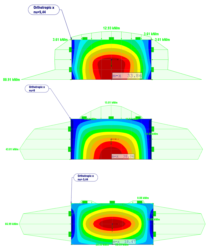
Results of Variation According to Table (Left: νxy = 5.44, Middle: νxy = 0, Right: νxy = -5.44)

With ν_xy = 0, the high amplitude of the support reaction at the free end of the plate is shifted to a constant value of 43 kN/m.

The moment m_x increases to 38.1 kNm/m. Compared to the previous result (ν_xy =5.44), the influence of the transversal strain is shown here. For ν = 0, no deformation or distortion is caused due to the transversal strain.

For ν_xy = −5.44, a post-critical failure is shown at the free plate end and the support reactions turn negative. The maximum moment occurs in the center of the plate with 59.5 kNm/m.

The plate now behaves more than a uniaxial stressed plate without the third support in the longitudinal direction.

This behavior can be explained with Image 01 and the relation listed there.

Due to the high negative transversal strain (ν_xy = −5.44), the plate is completely overpressed at the free edge and cannot, therefore, be deformed.

The influence of the orthotropy in the y-direction is almost zero here (E_y ≈ 0).

Conclusion

Almost any material parameters can be defined with the orthotropic material model in RFEM. Very different results are possible with the variation of the transversal strains. A transversal strain after modification of the values according to [1] results in values that lie close to the solution for a single-span beam.

Equation 31:

M_{y} = \frac{q l^{2}}{8} = 40 kNm

Formula 36

Overly high negative transversal strains show a modified structural system that no longer corresponds to the modeling.

Author

Mr. Kuhn is responsible for developing products for timber structures, and provides technical support for our customers.

Links

Nonlinear Structural Analysis Software

References

Huber, M. T : The Theory of Crosswise Reinforced Ferroconcrete Slabs and Its Application to Various Important Constructional Problems Involving Rectangular Slabs, Der Bauingenieur 12, Seiten 354 - 360, und 13, Seiten 392 - 395. 1923

Downloads

;