


Using RFEM, you have the capability to analyze various structural components such as member elements, plates, walls, shells, and solids. Prior to performing any calculations, it is necessary to generate a finite element (FE) mesh that corresponds to the desired 1D, 2D, and 3D elements.
The FE analysis involves breaking down the structural system into smaller subsystems, each represented by finite elements. Equilibrium conditions are established for each of these elements. This process leads to the formulation of a linear system of equations with numerous unknown variables. The precision of the results is directly influenced by the level of refinement in the mesh size of the finite elements. It is important to note that a finer mesh enhances accuracy, but it also increases computational time significantly due to the larger amount of data being processed. This is because additional equations need to be solved for every supplementary FE node.
Fortunately, the FE mesh is generated automatically by the software. Nonetheless, options exist that provide control over the mesh generation process.
1D Elements
Regarding member elements, the assumption is made that the cross-section maintains its planar shape during deformation. 1D member elements are employed to represent beams, trusses, ribs, cables, and rigid connections. Each 1D member element encompasses a total of twelve degrees of freedom – six at its initiation point and six at its terminal point. Those degrees of freedom pertain to displacements (ux, uy, uz) and rotations (φx, φy, φz).
If the torsional warping add-on is activated, an additional degree of freedom is available at each node, which can be used to take the warping into account.
In the context of linear structural analysis, tension, compression, and torsion are expressed as linear functions along the member axis (x), independent of bending and shear effects. This representation approximates these effects using a third-order polynomial in x, which also accounts for the influence of shearing stresses resulting from shear forces Vy and Vz. The stiffness matrix KL(12, 12) characterizes the linear behavior of these 1D elements. Additionally, for scenarios involving geometrically nonlinear problems where axial force interacts with bending, the stiffness matrix KNL(12, 12) is employed.
For precise calculations in cases involving significant deformations, it is advisable to enhance the accuracy of the finite element (FE) mesh for lines, as detailed in Chapter Line Mesh Refinements of the documentation.
2D Elements
Commonly, quadrilateral elements serve as 2D components in the structural analysis. The mesh generation process introduces triangular elements where they are needed. The degrees of freedom associated with the corner nodes of both quadrilateral and triangular elements align with those of 1D elements, encompassing displacement (ux, uy, uz) and rotation (φx, φy, φz). This arrangement ensures compatibility between 1D and 2D elements at nodes. The parameters are initially defined in the local planar coordinate system of the elements and subsequently transformed into the global coordinate system during the creation of the global stiffness matrix.
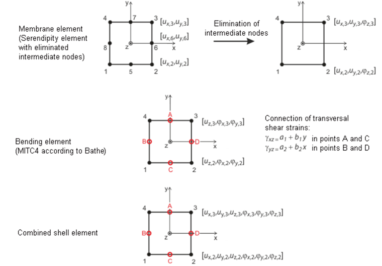
The planar shell elements are grounded in the Mindlin/Reissner theory. The graphical representation in the figure illustrates the element approaches. To directly link with member elements, a square approach is adopted within the shell plane (ux, uy). This choice eliminates intermediate nodes, resulting in a four-node element with an added degree of freedom φx. This configuration facilitates direct coupling between wall elements and beam elements. Additionally, MITC4 elements (Mixed Interpolation of Tensorial Components) as introduced by Dvorkin and Bathe [1] are employed. They rely on a mixed interpolation technique encompassing transversal deformations, cross-section rotations, and transversal shear strains.
At present, member elements are treated by solving the second-order analysis differential equation directly. However, when using the Saint Venant torsion, warping effects are not accounted for. The analysis of membranes is based on the Bergan principles. For instance, triangular elements are defined by breaking down the fundamental functions into three rigid-body deformations, three constant strain conditions, and three specific linear gradients of stress and strain. Within an element, the deformation field displays quadratic behavior, while the stress field maintains linearity. The element stiffness matrix KL is then transformed into nine combined parameters of the types ux, uy, φz. These matrix components are incorporated into the overall stiffness matrix (18, 18), alongside the components contributing to bending and shear effects, resulting in the Lynn/Dhillon concept.
Subsequently, the analysis involves the application of Mindlin plates, wherein plates with distinctive shear distortions are analyzed using Timoshenko's principles. This allows RFEM to correctly solve problems related to both thick and thin plates (Navier plates). In cases of geometrically nonlinear issues, the division of stress-strain conditions into a planar state and bending with shear interactions is not feasible. The interactions between these states are considered through the KNL matrix. RFEM utilizes a simplified yet effective version of the KNL matrix, influenced by Zienkiewicz's approaches. The square component ε2 of the Green/Lagrange strain tensor ε = ε1 + ε2 is employed. A linear distribution of uz(x, y) under the planar stress condition and linear distributions of ux(x, y) and uy(x, y) during bending interaction are assumed. This assumption is valid due to the primary impact of interaction being dependent on the first derivative of the differential equation and the rapid reduction in the influence of higher-order components with smaller element divisions. Numerous numerical analyses have validated the correctness of this approach.
When dealing with shell elements, it is essential for the thickness of the elements to be significantly smaller than their extension. If this condition is not met, it is advisable to model objects as solids instead. Furthermore, when utilizing shell elements, a gradual introduction of torsional stresses should be exercised, as the rotational degree of freedom about the surface normal is highly sensitive.
3D Elements
The following 3D elements are implemented in RFEM: tetrahedron, pentahedron (prism, pyramid), and hexahedron. Detailed information about applied elements and matrices can be found in Sevčík 3D Finite Elements with Rotational Degrees of Freedom (in Czech, available from Dlubal Software on request).
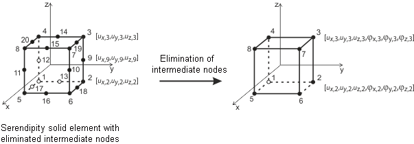
Generally, all rotational degrees of freedom must be regarded as critical for solids. As the deformation of a solid is solely determined from the displacement vectors, the rotation of a mesh node, for example due to singularly introduced torsion, does not affect the deformation within the solid.