55x

002022

Matthias Meyer, M.Sc.

2025-12-09

Temperature Loads on Bridges According to Eurocode

This article describes how to determine and combine temperature loads on bridges according to the Eurocode.

Standard Basis

The determination of temperature effects on bridges is regulated in EN 1991-1-5, Section 6 [1]. A distinction is initially made between temperature effects on the bridge superstructure (Section 6.1) and temperature effects on bridge piers (Section 6.2).

Temperature Effects on Bridge Superstructures

Bridge superstructures are classified into the following three types:

Type 1	Steel structures	Steel box girders, truss girders
Type 2	Composite structures
Type 3	Concrete structures	Concrete slabs, concrete girders, box girders

The temperature effect consists of a constant and a variable temperature component. [1]

Determination of Constant Temperature Component

The constant temperature component is determined according to EN 1991-1-5, Section 6.1.3 [1]. Depending on the superstructure type, the characteristic values for the minimum outside air temperature T_e,min and the maximum outside air temperature T_e,max are determined. The installation temperature T₀ is specified in the National Annex. If no information is available there, T₀ may be assumed to be 10°C. The characteristic value of the maximum negative change (shortening) T_N,con shall be assumed to be

{ΔT}_{N, con} = T_{0} - T_{e, \min}

T₀	Installation temperature
T_e,min	Characteristic value for the minimum constant temperature component

Calculation of Characteristic Value of Maximum Negative Change (Shortening)

The characteristic value of the maximum positive change (expansion) ∆T_N,exp shall be assumed to be

{ΔT}_{N, \exp} = T_{e, \max} - T_{0}

T_e,max	Characteristic value for the maximum constant temperature component
T₀	Installation temperature

Calculation of Characteristic Value of Maximum Positive Change (Expansion)

The total fluctuation of the constant temperature component is therefore calculated as follows:

{ΔT}_{N} = T_{e, \max} - T_{e, \min}

T_e,max	Characteristic value for the maximum constant temperature component
T_e,min	Characteristic value for the minimum constant temperature component

Calculation of Value of Total Temperature Change of Constant Temperature Component

Determination of Vertically Variable Temperature Component

Heating (for example, solar radiation during the day) and cooling (for example, contact with precipitation) of the upper component of the bridge superstructure result in a vertical temperature difference. This can induce stresses within the structure. Two methods are available for determining the vertically variable temperature component. The method to be used in a given country may be specified in the National Annex [1].

Method 1

Method 1 is described in EN 1991-1-5, Section 6.1.4.1 [1]. In this method, the vertical temperature difference is linear. If the top surface is warmer than the bottom side, a linear component with ∆_TM,heat is used. If the bottom side is warmer than the top side, a linear component with ∆subTM,cool is used. The values ∆T_M,heat and ∆T_M,cool are determined by the National Annex and depend on the superstructure type and the thickness of the top covering.

Method 2

Method 2 is described in Section 6.1.4.2 [1] and addresses the nonlinear effects on the vertical temperature component. The vertical temperature differences are specified in the National Annex and depend on the superstructure type and the structural system.

Determination of Horizontal Temperature Component

A horizontal temperature component should only be taken into account in exceptional cases [1].

Simultaneous Consideration of Constant and Variable Temperature Components

The simultaneous occurrence of constant and variable temperature loads can be interpreted as a load combination. The following expression is used to represent the combination of the two temperature loads:

{ΔT}_{M, heat} (or {ΔT}_{M, cool}) + ω_{N} {ΔT}_{N, \exp} (or {ΔT}_{N, con})

Combination of Temperature Action (Governing Variable Component)

ω_{M} {ΔT}_{M, heat} (or {ΔT}_{M, cool}) + {ΔT}_{N, \exp} (or {ΔT}_{N, con})

Combination of Temperature Action (Governing Constant Component)

In this case, the more unfavorable expression shall be selected. The numerical values for ω_N and ω_M are specified in the National Annex [1].

In the RFEM 6/RSTAB 9 model, it is necessary to create separate load cases for ∆T_N,exp, ∆T_N,con, ∆T_M,heat, and ∆T_M,cool. In the “Additional Settings” tab, you can then specify whether the temperature load is a constant (∆T_N) or a variable temperature component (∆T_M). Users have to make this setting manually. The “Additional Settings” tab only appears once at least two load cases of the “Temperature (Without Fire)” action category have been created.

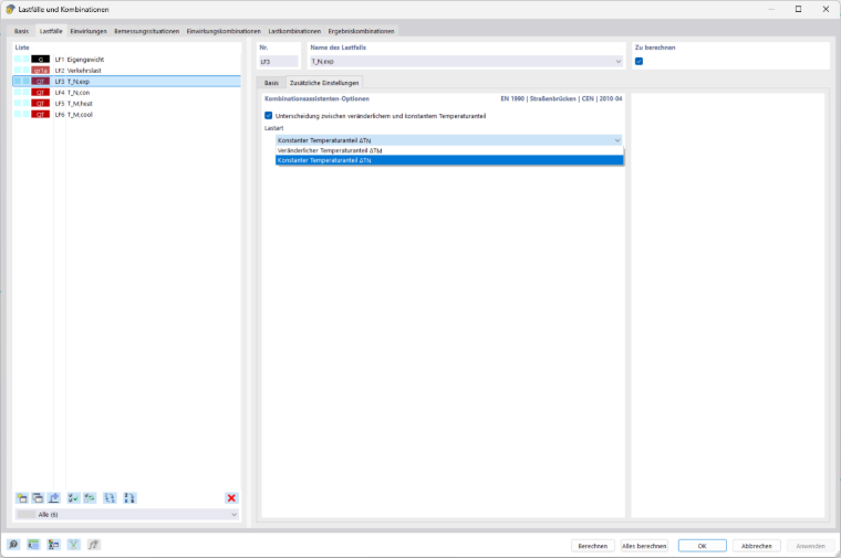
Editing window shows selection option for “Additional Settings” for loads of Temperature Load action category for bridges.

1 Selection of Variable or Constant Temperature Component

The combination wizard then generates 8 sub-load combinations from these 4 load cases, which are subsequently combined with the other load cases to form load combinations.

∆T_M,heat + ω_N · ΔT_N,exp
∆T_M,cool + ω_N · ΔT_N,exp
∆T_M,heat + ω_N · ΔT_N,con
∆T_M,cool + ω_N · ΔT_N,con
ω_M · ∆T_M,heat + ΔT_N,exp
ω_M · ∆T_M,cool + ΔT_N,exp
ω_M · ∆T_M,heat + ΔT_N,con
ω_M · ∆T_M,cool + ΔT_N,con

Info

The “Additional Settings” tab only appears if at least two temperature load cases have been generated. It is necessary to select the standard group “EN 1990 | Road Bridges” in the Base Data.

Application Example

In this application example, the values specified in the National Annexes are based on the recommended values of the European Committee for Standardization (CEN).

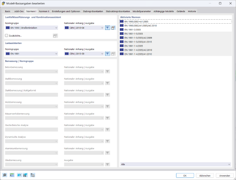
Editing window shows selection for Load Classification and Combination Wizard with National Annex as well as selection of Load Wizard with National Annex.

2 Selection of Standards I

The superstructure consists of a reinforced concrete slab (Type 3). For the characteristic outside air temperatures T_min and T_max, the values from DIN EN 1991-1-5 NA, NDP to 6.1.3.2 (1) [2] are used. The maximum and minimum constant temperature components are calculated according to the scheme recommended in Figure 6.1 [1]:

T_{e, \max} = T_{\max} + 2 ° C = 37 ° C + 2 ° C = 39 ° C

Calculation of Characteristic Value for Maximum Constant Temperature Component

T_{e,min} = T_{\min} + 8 ° C = - 24 ° C + 8 ° C = - 16 ° C

Characteristic Value for Minimum Constant Temperature Component

The default value used is T₀ = 10°C, as recommended in DIN EN 1991-1-5, Section 6.1.3.3 [1]. This results in the following values for the constant temperature components:

{ΔT}_{N, con} = T_{0} - T_{e, \min} = 10 ° C - (- 16 ° C) = 26 ° C

Example Calculation of Characteristic Value of Maximum Negative Change (Shortening)

{ΔT}_{N, \exp} = T_{e, \max} - T_{0} = 37 ° C - 10 ° C = 27 ° C

Example Calculation of Characteristic Value of Maximum Positive Change (Strain)

When ∆T < sub> N,con < /sub>, this represents the maximum negative change. Accordingly, it is necessary to apply a constant temperature load of T < sub> c = –26 °C in the model.

The linearly varying component is determined according to Method 1. The recommended values according to EN 1991-1-5, Table 6.1 [2] are used and multiplied by a factor k_sur to take into account different covering thicknesses according to EN 1991-1-5, Table 6.2 [2]. For Superstructure Type 3 (concrete structure—plate) without a covering, the variable temperature component for the “Top side warmer than bottom side” load case ∆T _M,heat and the variable temperature component for the “Bottom side warmer than top side” load case ∆T _M,cool are calculated as follows:

{ΔT}_{M, heat} = 15 ° C \cdot k_{sur} = 15 ° C \cdot 0.8 = 12 ° C

Example Calculation of Variable Temperature for Case of Top Side Warmer Than Bottom Side

{ΔT}_{M, cool} = 8 ° C \cdot k_{sur} = 8 ° C \cdot 1.1 = 8.8 ° C

Example Calculation of Variable Temperature Component for Case of Bottom Side Warmer Than Top Side

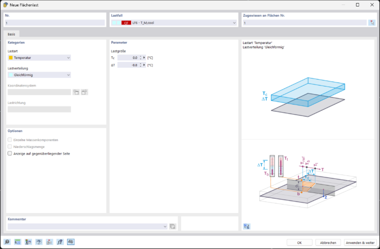
These values, including the top covering thickness factor k_sur need to be determined by the user and then applied as a linear temperature load. The vertical temperature distribution for the load case T_M,cool should increase linearly from top to bottom. Accordingly, a linear temperature load of ∆T = –8.8 °C shall be applied in the model for this load case.

According to the CEN recommendations in Eurocode 0 [3], the partial safety factor for temperature loads on road bridges is γ_Q = 1.5, and the combination coefficient is ψ₀ = 0.6.

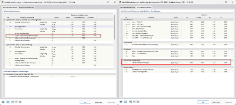
Editing window shows partial safety factors and combination coefficients for EN 1990 | Road Bridges | CEN | 2010-04.

3 View of Partial Safety Factors and Combination Coefficients

To take into account both constant and variable temperature components simultaneously, the recommended values ω_N = 0.35 and ω_M = 0.75 according to EN 1991-1-5, Section 6.1.5 [2] apply. The values depend on the National Annex selected for the load wizard (Image 2).

For the temperature components

∆T_N,con (T_c = –26 °C, ∆T = 0)
∆T_N,exp (T_c = 27 °C, ∆T = 0)
∆T_M,heat (T_c = 0, ∆T = 12 °C)
∆T_M,cool (T_c = 0, ∆T = -8.8°C),

separate load cases are created, and in each load case, a “Temperature” surface load is applied to the superstructure surface. In this application example, the self-weight (Load Case 1) is also taken into account, and a live load (Load Case 2) is applied.

The editing window shows new uniform temperature load.

4 View of Temperature Load Type with Uniform Load Distribution

The load cases ∆T_N,con and ∆T_N,exp are defined as a constant temperature component T_N according to Image 1. The load cases ∆T_M,heat and ∆T_M,cool are defined as a variable temperature component T_M according to Image 1.

If the combination wizard is activated, constant and variable temperature components are automatically combined with the other load cases. The values ω_N and ω_M are incorporated into the scalar factors. Together with the partial safety factor and any combination coefficient, the sub-load combinations described in the previous chapter are then created.

(ψ₀ + γ_Q,T) · (ω_N · ΔT_N,exp + ∆T_M,heat)
(ψ₀ + γ_Q,T) · (ΔT_N,exp + ω_M · ∆T_M,heat)
(ψ₀ + γ_Q,T) · (ω_N · ΔT_N,exp + ∆T_M,cool)
(ψ₀ + γ_Q,T) · (ΔT_N,exp + ω_M · ∆T_M,cool)
(ψ₀ + γ_Q,T) · (ω_N · ΔT_N,con + ∆T_M,heat)
(ψ₀ + γ_Q,T) · (ΔT_N,con + ω_M · ∆T_M,heat)
(ψ₀ + γ_Q,T) · (ω_N · ΔT_N,con + ∆T_M,cool)
(ψ₀ + γ_Q,T) · (ΔT_N,con + ω_M · ∆T_M,cool)

with ψ₀=0.6; γ_Q,T=1.5; ω_N=0.35 and ω_M=0.75

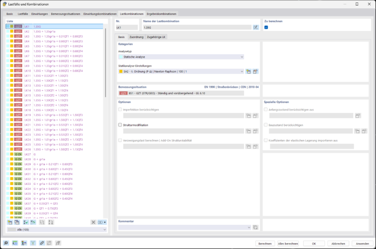
The sub-load combinations are then combined with the other load cases to obtain load combinations (Image 5).

As an example, Load Combination 3 in Figure 5 is modeled in detail:

E_{d} = γ_{G} \cdot G_{k} + γ_{Q, 1} \cdot P_{k} + ψ_{0} \cdot γ_{Q, T} \cdot ω_{N} \cdot ∆ T_{N, \exp} + ψ_{0} \cdot γ_{Q, T} \cdot ∆ T_{M, heat} = 1.35 G_{k} + 1.35 P_{k} + 0.6 \cdot 1.5 \cdot 0.35 \cdot ∆ T_{N, \exp} + 0.6 \cdot 1.5 \cdot ∆ T_{M, heat} = 1.35 G_{k} + 1.35 P_{k} + 0.31 ∆ T_{N, \exp} + 0.9 ∆ T_{M, heat}

Example Composition of Load Combination 3

Editing window shows generated load combinations.

5 View of Editing Window of Load Cases and Combinations

Constant Temperature Difference Between Different Structural Components

Unfavorable stresses resulting from different constant temperature components between different structural components should also be taken into account. For example, different constant temperature components may arise between light-colored and dark-colored structural components. These stresses shall be applied in addition to the constant temperature components. The values for the different constant temperature components are specified in the National Annex. [1]

Temperature Effects on Bridge Piers

It is necessary to consider the temperature effects on bridge piers if they cause constraint forces or movements in the connected structures. For piers and walls, a linearly varying temperature difference between the outer sides needs to be assumed. The temperature differences are specified in the National Annex. [2]

Author

Matthias works in Product Engineering, specializing in timber structures, and also assists with quality assurance and customer support.

References

DIN. (2010). Eurocode 1: Actions on Structures – Part 1‑5: General Actions – Temperature Actions. Berlin, Beuth Verlag GmbH.
DIN. (2010). National Annex – Nationally Determined Parameters – Eurocode 1: Actions on Structures – Part 1-5: General Actions – Thermal Actions. Berlin, Beuth Verlag GmbH.
Deutsches Institut für Normung e.V. (DIN). (2010). Eurocode 0: Basis of Structural Design; DIN EN 1990:2010-12. Berlin, DIN.

;