Time-Dependent Deflection Analysis of Reinforced Concrete Members According to ACI 318 Considering Long-Term Effects (Creep and Shrinkage per ACI 435)

I. Input Data

1. Geometry

System: Single-span beam
Span: l = 12 ft
Cross-section Width: b = 93.0 in
Cross-section Height: h = 6.0 in
Effective depth: d = 6 – 0.650 – 0.3125 = 5.0375 in

2. Materials

• Concrete

Concrete compressive strength: f’c = 3,000 ksi
Modulus of elasticity: E = 3,122.019 ksi

To consider creep and shrinkage, the time-dependent properties of concrete need to be activated:

These properties are now set for all members and surfaces with this material assigned. It is however possible to edit these properties for specific a member by editing these properties in the cross-section options of that member:

• Reinforcing Steel

Specified yield strength: fy = 40,000 ksi
Modulus of elasticity: Es = 29,000.0 ksi
Reinforcement quantity: 11 bars with 0.625 in diameter
Reinforcement area: As,prov = 3.37 in²
Reinforcement ratio: ρ = 0.60%

3. Serviceability Configuration

For time-dependent deflection, creep and shrinkage can be considered using two different approaches:

• Time-dependent factor according to Table 24.2.4.1.3
• Time-dependent material properties (creep and shrinkage) according to ACI 435

This example uses the second approach; therefore, it is selected in the serviceability configuration:

4. Load Cases and Combinations

The load case action categories are defined in accordance with ASCE 7.

• Load Case 1 (LC1)

Action Category: Dead Load (D)
Load Case 1 includes the self-weight of the member and an additional uniformly distributed member load with a magnitude of 0.8 kip/ft.

• Load Case 2 (LC2)

Action Category: Live Load (L)
Load Case 2 consists of a uniformly distributed member load with a magnitude of 1.6 kip/ft.

• Design Situations

For deflection analysis, a design situation is created based on ASCE 7 Section 2.4 (ASD) using unfactored load combinations. The load combination wizard is activated for this design situation to automatically generate load combinations.

• Load Combinations

Two load combinations are generated:

• CO1: LC1
• CO2: LC1 + LC2

In deflection analysis, creep and shrinkage in reinforced concrete are caused only by long-term, sustained loads, such as the self-weight of the structure. Short-term loads, such as live loads, generally do not contribute significantly to these time-dependent effects.
To accurately capture creep and shrinkage, it is essential to define sustained long-term loads in the analysis. The deflections resulting from these sustained loads are then calculated and subsequently included in the total deflection when evaluating the relevant load combinations. This ensures that the long-term behavior of the structure is properly considered in the serviceability assessment.
To account for these effects in the concrete add-on calculation, a separate design situation must be created. This design situation is based on ASCE 7 Section 2.4 (ASD). No combination wizard is assigned, as the load combination will be created manually, allowing precise control over which sustained long-term loads contribute to creep and shrinkage.

To indicate to the concrete design add-on which design situation includes the long-term sustained load combination, the limit state type of the design situation is set to Serviceability Design | Long-Term Sustained.

A load combination with the new design situation (DS2) is then created. In this example, only the self-weight is assumed to act as the long-term sustained load contributing to creep and shrinkage. Therefore, a load combination including only the self-weight (LC1) is defined to capture the time-dependent effects accurately.

The created load combination CO3 is then used to calculate the long-term deflection of the member due to the sustained load. To include this deflection when evaluating the total deflection, CO3 is assigned as the corresponding load combination (CO) for the two load combinations of DS2.

With the corresponding load assigned, crack state detection in the serviceability configuration is set to “Crack state from corresponding CO of SLS design situation from associated load”. This ensures that the distribution coefficient ζd is calculated as the maximum value across all corresponding loads.

II. Concrete Design Calculation

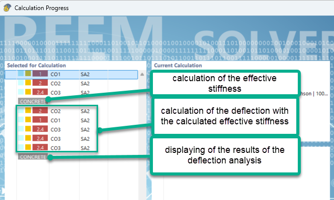
For deformation analysis in the Concrete Design add-on, an analytical method is used for 2D structures and 1D elements that are subjected to axial forces and bending moments. This is based on the determination of effective stiffnesses (effective stiffness method) on the cross-section plane, taking into account the crack state as well as effects like tension stiffening and simple long-term effect.

1. Calculating Deflection Due to Long-Term Sustained Load

a. Curvature for uncracked state

This section presents the calculation of the long-term deflection of the member under CO3 (self-weight, including the effects of creep and shrinkage). The design check is carried out at the critical location x = 6.0 ft, where only a flexural moment of M_y,u = 14.40 kipft is present. The axial force at this location is P_u = 0.

Creep effects are accounted for by reducing the modulus of elasticity. The influence of creep is incorporated using the ultimate creep coefficient 𝜑:
Effective Modulus of Elasticity of Concrete:
\(\mathrm{E_{c,eff}} = \dfrac{\mathrm{E_{c}}}{1 + \phi}\)
\(\mathrm{E_{c,eff}} = \dfrac{3122.020\,\mathrm{ksi}}{1 + 3.200} = 743.319\,\mathrm{ksi}\)

Effective Modular Ratio:
\(\alpha_{e} = \dfrac{E_{s}}{E_{c,eff}}\)
\(\alpha_{e} = \dfrac{29000.000\,\mathrm{ksi}}{743.319\,\mathrm{ksi}} = 39.01\)

Effective Modular Ratio (short-term loading):
\(\alpha_{e,st} = \dfrac{E_{s}}{E_{c}}\)
\(\alpha_{e,st} = \dfrac{29000.000\,\mathrm{ksi}}{3122.020\,\mathrm{ksi}} = 9.29\)

The effective modular ratios are used to calculate the geometrical parameters for the uncracked state (short- and long-term) and the cracked state:

State I - Uncracked State
Description	Symbol	Value	Unit
Distance of center of gravity of ideal section from concrete surface in compression (determined for uncracked state)	zI	3.389	in
Effective section area in uncracked state	AI	689.664	in2
Effective moment of inertia to ideal center of gravity in uncracked state	Iy,I	2116.230	in4
Eccentricity of ideal center of gravity of section in uncracked state	ez,I	0.389	in

State I - Uncracked state - Short-term loading
Description	Symbol	Value	Unit
Distance of center of gravity of ideal section from concrete surface in compression (determined for uncracked state)	zI,st	3.108	in
Effective section area in uncracked state	AI,st	589.348	in2
Effective moment of inertia to ideal center of gravity in uncracked state	Iy,I,st	1797.210	in4

Shrinkage:
Shrinkage causes an additional axial force in the reinforcement. Due to the eccentricity of the reinforcement to the center of gravity of the ideal section, an additional curvature caused by shrinkage is present.

The additional force due to shrinkage is then calculated:
\( \mathrm{P_{sh}} = - \mathrm{E_{s}} \cdot \varepsilon_{\mathrm{sh}} \cdot \left( \mathrm{A_{s,def,+z (bottom)}} + \mathrm{A_{s,def,-z (top)}} \right) \)

\( \mathrm{P_{sh}} = -29000.000\,\mathrm{ksi} \cdot -0.600000\,\text{‰} \cdot \left( 3.37\,\mathrm{in^2} + 0.00\,\mathrm{in^2} \right) = 58.721\,\mathrm{kip} \)

The eccentricity of the shrinkage force to t he center of gravity of the ideal section in the uncracked state is then:

\(\mathrm{e_{sh,z,I}} = \dfrac{A_{s,def,+z (bottom)} \cdot d_{def,+z (bottom)} + A_{s,def,-z (top)} \cdot d_{def,-z (top)}}{A_{s,def,+z (bottom)} + A_{s,def,-z (top)}} - \mathrm{z_{I}}\)

\(\mathrm{e_{sh,z,I}} = \dfrac{3.37\,\mathrm{in^2} \cdot 5.037\,\mathrm{in} + 0.00\,\mathrm{in^2} \cdot 3.000\,\mathrm{in}}{3.37\,\mathrm{in^2} + 0.00\,\mathrm{in^2}} - 3.389\,\mathrm{in} = 1.649\,\mathrm{in}\)

As a result the Bending moment caused by axial force P_sh:
\(\mathrm{M_{sh,y,I}} = \mathrm{P_{sh}} \cdot \mathrm{e_{sh,z,I}}\)

\(\mathrm{M_{sh,y,I}} = 58.721\,\mathrm{kip} \cdot 1.649\,\mathrm{in} = 8.07\,\mathrm{kipft}\)

A curvature coefficient for the uncracked state is then determined. It indicates how the shrinkage moment acts relative to the axial force and its eccentricity. It shows how the distribution of shrinkage forces and the location of the centroid influence the deformations of the element. This value is crucial for fully describing the cross-sectional deformations caused by shrinkage:
\(\mathrm{k_{sh,y,I}} = \dfrac{\mathrm{M_{sh,y,I}} + \mathrm{M_{y,Ed,def}} - \mathrm{P_{u}} \cdot \mathrm{e_{z,I}}}{\mathrm{M_{y,Ed,def}} - \mathrm{P_{u}} \cdot \mathrm{e_{z,I}}}\)

\(\mathrm{k_{sh,y,I}} = \dfrac{8.07\,\mathrm{kipft} + 14.40\,\mathrm{kipft} - 0.000\,\mathrm{kip} \cdot 0.389\,\mathrm{in}}{14.40\,\mathrm{kipft} - 0.000\,\mathrm{kip} \cdot 0.389\,\mathrm{in}} = 1.560\)

The total curvature for the uncracked state can now be calculated:

\(\kappa_{y,I} = \mathrm{k_{sh,y,I}} \cdot \dfrac{\mathrm{M_{y,Ed,def}} - \mathrm{P_{u}} \cdot \mathrm{e_{z,I}}}{E_{c,eff} \cdot \mathrm{I_{y,I}}}\)
\(\kappa_{y,I} = 1.560 \cdot \dfrac{14.40\,\mathrm{kipft} - 0.000\,\mathrm{kip} \cdot 0.389\,\mathrm{in}}{743.319\,\mathrm{ksi} \cdot 2116.230\,\mathrm{in^4}} = 2.1\,\mathrm{mrad/ft}\)

b. Curvature for Cracked State

State II - Cracked state -
Description	Symbol	Value	Unit
Depth of compression zone in cracked state	cII	2.618	in
Distance of center of gravity of ideal section from concrete surface in compression (determined for cracked state)	zII	2.618	in2
Effective section area in cracked state	AII	375.100	in2
Effective moment of inertia to ideal center of gravity in cracked state	Iy,II	1326.990	in4
Eccentricity of ideal center of gravity of section in cracked state	ez,II	-0.382	in

Shrinkage - Cracked state
Description	Symbol	Value	Unit
Eccentricity of shrinkage force to center of gravity of ideal section in cracked state	esh,z,II	2.420	in
Bending moment caused by axial force Nsh for cracked state	Msh,y,II	11.84	kipft
Curvature coefficient for cracked state	ksh,y,II	1.822	-

\(\kappa_{y,II} = \mathrm{k_{sh,y,II}} \cdot \dfrac{\mathrm{M_{y,Ed,def}} - \mathrm{P_{u}} \cdot \mathrm{e_{z,II}}}{E_{c,eff} \cdot \mathrm{I_{y,II}}}\)
\(\kappa_{y,II} = 1.822 \cdot \dfrac{14.40\,\mathrm{kipft} - 0.000\,\mathrm{kip} \cdot (-0.382\,\mathrm{in})}{743.319\,\mathrm{ksi} \cdot 1326.990\,\mathrm{in^4}} = 3.8\,\mathrm{mrad/ft}\)

c. Curvature for Uncracked and Cracked States

The maximum stress in the uncracked state under short-term and long-term loading is calculated and then compared. The greater of the two values is used to determine the distribution coefficient.

Maximum stress in uncracked state
Description	Symbol	Value	Unit
Maximum stress in uncracked state (long-term loading)	fmax,lt	0.418	ksi
Maximum stress in uncracked state (short-term loading)	fmax,st	0.278	ksi

The distribution factor is calculated using the following formula:
\(\zeta_{d} = 1 - \left( \dfrac{\dfrac{2}{3} \cdot f_{r}}{f_{max}} \right)^2\)
\(\zeta_{d} = 1 - \left( \dfrac{\dfrac{2}{3} \cdot 0.411\,\mathrm{ksi}}{0.418\,\mathrm{ksi}} \right)^2 = 0.570\)

\(\kappa_{y,f} = \zeta_{d} \cdot \kappa_{y,II} + (1 - \zeta_{d}) \cdot \kappa_{y,I}\)
\(\kappa_{y,f} = 0.570 \cdot 3.8\,\mathrm{mrad/ft} + (1 - 0.570) \cdot 2.1\,\mathrm{mrad/ft} = 3.1\,\mathrm{mrad/ft}\)

d. Final Stiffness

Using the obtained distribution coefficient together with the cross-section parameters in the cracked and uncracked states, the effective cross-section parameters can now be determined:

Effective cross-section parameters
Description	Symbol	Value	Unit
Ideal section area	Af	466.537	in2
Ideal moment of inertia to ideal center of section	Iy,f	909.112	in4
Eccentricity of centroid	ez,f	-0.135	in
Ideal moment of inertia to geometric center of section	Iy,0,f	917.601	in4

Since, in this example, the only internal force present is the flexural moment, only the tangent bending stiffness is relevant:

\(\mathrm{EI_{y,0,f}} = E_{c,eff} \cdot \mathrm{I_{y,0,f}}\)
\(\mathrm{EI_{y,0,f}} = 743.319\,\mathrm{ksi} \cdot 917.601\,\mathrm{in^4} = 4736.60\,\mathrm{kipft^2}\)

With the newly calculated effective stiffness, a new statical analysis is then carried out to obtain the deflection:

A vertical deflection of 0.420 in is obtained at the midspan of the beam.

The limit deflection is defined as:
\(\mathrm{u_{z,lim}} = \dfrac{L_{z,ref}}{L_{z,ref} / u_{z,lim}}\)

\(\mathrm{u_{z,lim}} = \dfrac{12.00\,\mathrm{ft}}{240.000} = 0.600\,\mathrm{in}\)

Based on this, the design check ratio is calculated as:
\(\eta = \left|\dfrac{u_{z}}{u_{z,lim}}\right|\)

\(\eta = \left|\dfrac{0.420\,\mathrm{in}}{0.600\,\mathrm{in}}\right| = 0.701\)

2. Calculating the Total Deflection Load

For the total deflection, CO2 (LC1 + LC2) is the governing load combination. A bending moment of 43.20 kipft is present.
Since only sustained loads cause creep and shrinkage, creep effects are not considered when calculating cross-section properties for short-term loads. Therefore, the effective modulus of elasticity of concrete E_c is used for the calculation, and the shrinkage curvature coefficient is set to 1.0.

a. Curvature for Uncracked State

The geometrical parameters in the uncracked state correspond to the short-term geometrical parameters of the sustained load:

State I - Uncracked state
Description	Symbol	Value	Unit
Distance of center of gravity of ideal section from concrete surface in compression (determined for uncracked state)	zI	3.108	in
Effective section area in uncracked state	AI	589.348	in2
Effective moment of inertia to ideal center of gravity in uncracked state	Iy,I	1797.210	in4
Eccentricity of ideal center of gravity of section in uncracked state	ez,I	0.108	in

The curvature in the uncracked state is then calculated:
\(\kappa_{y,I} = k_{sh,y,I} \cdot \frac{M_{y,Ed,def} - P_{u} \cdot e_{z,I}}{E_{c,eff} \cdot I_{y,I}} \)

\(\kappa_{y,I} = 1.000 \cdot \frac{43.20\,\text{kipft} - 0.000\,\text{kip} \cdot 0.108\,\text{in}}{3122.020\,\text{ksi} \cdot 1797.210\,\text{in}^4} = 1.1\,\text{mrad/ft}\)

b. Curvature for Cracked State

The geometric parameters in the cracked state for short-term loads are determined without considering the creep effects:

State II - cracked state
Description	Symbol	Value	Unit
Depth of compression zone in cracked state	cII	1.536	in
Distance of center of gravity of ideal section from concrete surface in compression (determined for cracked state)	zII	1.536	in
Effective section area in cracked state	AII	174.226	in2
Effective moment of inertia to ideal center of gravity in cracked state	Iy,II	496.674	in4

The curvature in the cracked state is then calculated:
\(\kappa_{y,II} = k_{sh,y,II} \cdot \frac{M_{y,Ed,def} - P_{u} \cdot e_{z,II}}{E_{c,eff} \cdot I_{y,II}}\)

\(\kappa_{y,II} = 1.000 \cdot \frac{43.20\,\text{kipft} - 0.000\,\text{kip} \cdot (-1.464)\,\text{in}}{3122.020\,\text{ksi} \cdot 496.674\,\text{in}^4} = 4.0\,\text{mrad/ft}\)

c. Curvature from uncracked and cracked states

For the calculation of the distribution factor, the maximum stress in the uncracked state for this cross-section is required:
\(f_{max} = \frac{P_{u}}{A_{I}} + \frac{M_{y,Ed,def} - P_{u} \cdot \left( z_{I} - \frac{h}{2} \right)}{I_{y,I}} \cdot \left( h - z_{I} \right)\)

The resulting distribution factor is then:
\(f_{max} = \frac{0.000\,\text{kip}}{589.348\,\text{in}^2} + \frac{43.20\,\text{kipft} - 0.000\,\text{kip} \cdot \left( 3.108\,\text{in} - \frac{6.000\,\text{in}}{2} \right)}{1797.210\,\text{in}^4} \cdot \left( 6.000\,\text{in} - 3.108\,\text{in} \right) = 0.834\,\text{ksi}\)

The final curvature is finally calculated:
\(\kappa_{y,f} = \zeta_{d} \cdot \kappa_{y,II} + \left( 1 - \zeta_{d} \right) \cdot \kappa_{y,I}\)

\(\kappa_{y,f} = 0.892 \cdot 4.0\,\text{mrad/ft} + \left( 1 - 0.892 \right) \cdot 1.1\,\text{mrad/ft} = 3.7\,\text{mrad/ft}\)

d. Final Stiffness

The effective cross-section parameters can now be determined:

Effective cross-section parameters
Description	Symbol	Value	Unit
Ideal section area	Af	188.543	in2
Ideal moment of inertia to ideal center of section	Iy,f	538.700	in4
Eccentricity of centroid	ez,f	-1.413	in
Ideal moment of inertia to geometric center of section	Iy,0,f	915.074	in4

The bending
fness can now be calculated:
\(EI_{y,0,f} = E_{c,eff} \cdot I_{y,0,f}\)

\(EI_{y,0,f} = 3122.020\,\text{ksi} \cdot 915.074\,\text{in}^4 = 19839.40\,\text{kipft}^2\)

Using the calculated effective stiffness, the short-term total deflection is calculated. A deflection of 0.984 is reached.

The calculation of the total deflection of the beam under frequent loads requires consideration of the different deformation components resulting from various load types and their respective effects on the member. Long-term and short-term deformations must be treated separately in order to determine the actual deflection correctly:

\(u_{z,tot} = u_{z,QP,lt} + \left( u_{z,tot,st} - u_{z,QP,st} \right)\)

• u_z,QP,lt: This deflection is caused by long-term sustained loads and takes into account the creep effects that the member will experience over a long period of time. This is the deflection calculated in Section 1.

• u_z,tot,st: Short-term total deflection. This deformation occurs immediately after the application of the frequent load. This is the deflection calculated in this section.

• u_z,QP,st: Short-term total deflection of the long-term sustained loads. This deformation develops directly after the application of sustained loads and represents the instantaneous response of the member before creep effects occur.

The total deflection u_z,tot consists of the long-term deflection u_z,QP,lt due to long-term sustained loads and the additional deflection from short-term effects. This additional deflection is calculated as the difference between the total short-term deflection u_z,tot,st and the short-term deflection caused by the creep-inducing loads u_z,QP,st. The following graphic illustrates this clearly:

\(u_{z,tot} = u_{z,QP,lt} + \left( u_{z,tot,st} - u_{z,QP,st} \right)\)

\(u_{z,tot} = 0.420\,\text{in} + \left( 0.630\,\text{in} - 0.067\,\text{in} \right) = 0.984\,\text{in}\)

\(\eta = \left|\dfrac{0.984\,\mathrm{in}}{0.600\,\mathrm{in}}\right| = 1.640 >1 \)
In this case, the total deflection is higher than the limit and the design check is not fulfilled.

In summary, this example demonstrates the comprehensive calculation of reinforced concrete beam deflections considering both short-term and long-term effects, including creep and shrinkage. Using the RFEM Concrete Design add-on, the beam’s effective stiffness was determined through an analytical method accounting for uncracked and cracked states, tension stiffening, and time-dependent material properties. The long-term deflection due to sustained loads was first calculated (0.420 in), followed by the total short-term deflection under frequent loads (0.984 in). When combined, the total deflection (0.984 in) exceeds the allowable limit (0.600 in), resulting in a design check ratio of 1.64, indicating that the beam does not satisfy serviceability requirements. This highlights the critical importance of accurately modeling time-dependent concrete behavior and load combinations in serviceability analysis.