- Consideration of 7 local deformation directions (ux, uy, uz, φx, φy, φz, ω) or 8 internal forces (N, Vu, Vv, Mt,pri, Mt,sec, Mu, Mv, Mω) when calculating member elements
- Usable in combination with a structural analysis according to linear static, second-order, and large deformation analysis (imperfections can also be taken into account)
- In combination with the Stability Analysis add-on, allows you to determine critical load factors and mode shapes of stability problems such as torsional buckling and lateral-torsional buckling
- Consideration of end plates and transverse stiffeners as warping springs when calculating I-sections with automatic determination and graphical display of the warping spring stiffness
- Graphical display of the cross-section warping of members in the deformation
- Full integration with RFEM and RSTAB

You can perform the calculation of the warping torsion on the entire system. Thus, you consider the additional 7th degree of freedom in the member calculation. The stiffnesses of the connected structural elements are automatically taken into account. It means, you don't need to define equivalent spring stiffnesses or support conditions for a detached system.
You can then use the internal forces from the calculation with warping torsion in the add-ons for the design. Consider the warping bimoment and the secondary torsional moment, depending on the material and the selected standard. A typical application is the stability analysis according to the second-order theory with imperfections in steel structures.
Did you know that The application is not limited to thin-walled steel cross-sections. Thus, it is possible for you, for example, to perform the calculation of the ideal overturning moment of beams with solid timber cross-sections.

- You can activate or deactivate the use of torsional warping in the Add-ons tab of the model's Base Data.
- After activating the add-on, the user interface in RFEM is extended by some new entries in the navigator, tables, and dialog boxes.
- Simple definition of construction stages in the RFEM structure including visualization
- Adding, removing, modifying, and reactivating member, surface, and solid elements and their properties (for example, member and line hinges, degrees of freedom for supports, and so on)
- Automatic and manual combinatorics with load combinations in the individual construction stages (for example, to consider mounting loads, mounting cranes, and other loads)
- Consideration of nonlinear effects such as tension member failure or nonlinear supports
- Interaction with other add-ons, such as Nonlinear Material Behavior, Structure Stability, Form-Firnding, and so on.
- Display of results numerically and graphically for individual construction stages
- Detailed printout report with documentation of all structural and load data for each construction stage

Have you created the entire structure in RFEM? Very well, now you can assign the individual structural components and load cases to the corresponding construction stages. In each construction stage, you can modify release definitions of members and supports, for example.
You can thus model structural modifications, such as those that occur when bridge girders are successively grouted or when columns are settled. Then, assign the load cases created in RFEM to the construction stages as permanent or non-permanent loads.
Did you know that The combinatorics allows you to superimpose the permanent and non-permanent loads in load combinations. In this way, it is possible for you to determine the maximum internal forces of different crane positions or to consider temporary mounting loads available in one construction stage only.

If there are geometry differences arising between the ideal and the deformed structural system from the previous construction stage, they are compared in the program. The next construction stage is built on top of the stressed system from the previous construction stage. This calculation is nonlinear.

Was the calculation successful? Now you can view the results of the individual construction stages graphically and in tables in RFEM. Moreover, RFEM allows you to consider the construction stages in the combinatorics and include it in further design.

- Automatic consideration of masses from self-weight
- Direct import of masses from load cases or load combinations
- Optional definition of additional masses (nodal, linear, or surface masses, as well as inertia masses) directly in the load cases
- Optional neglect of masses (for example, mass of foundations)
- Combination of masses in different load cases and load combinations
- Preset combination coefficients for various standards (EC 8, SIA 261, ASCE 7,...)
- Optional import of initial states (for example, to consider prestress and imperfection)
- Structure Modification
- Consideration of failed supports or members/surfaces/solids
- Definition of several modal analyses (for example, to analyze different masses or stiffness modifications)
- Selection of mass matrix type (diagonal matrix, consistent matrix, unit matrix), including user-defined specification of translational and rotational degrees of freedom
- Methods for determining the number of mode shapes (user-defined, automatic - to reach effective modal mass factors, automatic - to reach the maximum natural frequency - only available in RSTAB)
- Determination of mode shapes and masses in nodes or FE mesh points
- Results of eigenvalue, angular frequency, natural frequency, and period
- Output of modal masses, effective modal masses, modal mass factors, and participation factors
- Masses in mesh points displayed in tables and graphics
- Visualization and animation of mode shapes
- Various scaling options for mode shapes
- Documentation of numerical and graphical results in printout report

In the modal analysis settings, you have to enter all data that are necessary for the determination of the natural frequencies. These are, for example, mass shapes and eigenvalue solvers.
The Modal Analysis add-on determines the lowest eigenvalues of the structure. Either you adjust the number of eigenvalues or let them determined automatically. Thus, you should reach either effective modal mass factors or maximum natural frequencies. Masses are imported directly from load cases and load combinations. In this case, you have the option to consider the total mass, load components in the global Z-direction, or only the load component in the direction of gravity.
You can manually define additional masses at nodes, lines, members, or surfaces. Furthermore, you can influence the stiffness matrix by importing axial forces or stiffness modifications of a load case or load combination.

In RFEM, you can use these three powerful eigenvalue solvers:
- Root of Characteristic Polynomial
- Method by Lanczos
- Subspace Iteration
RSTAB, on the other hand, provides you with these two eigenvalue solvers:
- Subspace Iteration
- Shifted inverse power method
The selection of the eigenvalue solver depends primarily on your model size.

As soon as the program has completed the calculation, the eigenvalues, natural frequencies and periods are listed. These result windows are integrated in the main program RFEM/RSTAB. You can find all mode shapes of the structure in tables and also have an option to display them graphically and to animate them.
All result tables and graphics are part of the RFEM/RSTAB printout report. In this way, you can ensure clearly arranged documentation. You can also export the tables to MS Excel.

- Stress determination using an elastic-plastic material model
- Design of masonry disc structures for compression and shear on the building model or single model
- Automatic determination of stiffness of a wall-slab hinge
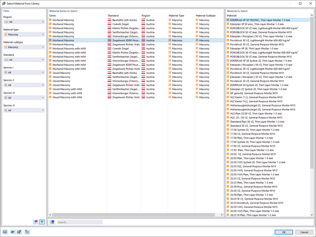
- An extensive material database for almost all stone-mortar combinations available on the Austrian market (the product range is continuously being expanded, for other countries as well)
- Automatic determination of material values according to Eurocode 6 (ÖN EN 1996‑X)
- Option to create pushover analysis
You enter and model the structure directly in RFEM. You can combine the masonry material model with all common RFEM add-ons. This enables you to design the entire building models in connection with masonry.
The program automatically determines for you all parameters required for the calculation by using the material data that you have entered. Then, it finally generates the stress-strain curves for each FE element.

Was your design successful? Then just sit back and relax. You benefit from the numerous functions in RFEM also here. The program gives you the maximum stresses of the masonry surfaces, whereby you can display the results in detail at each FE mesh point.
Moreover, you can insert sections in order to carry out a detailed evaluation of the individual areas. Use the display of the yield areas to estimate the cracks in the masonry.
Compared to the RF‑/STAGES add-on module (RFEM 5), the following new features have been added to the Construction Stages Analysis (CSA) add-on for RFEM 6:
- Consideration of construction stages at RFEM level
- Integration of the construction stage analysis into the combinatorics in RFEM
- Additional structural elements, such as line hinges, are supported
- Analysis of alternative construction processes in a model
- Reactivation of elements
Compared to the RF-/STEEL Warping Torsion add-on module (RFEM 5 / RSTAB 8), the following new features have been added to the Torsional Warping (7 DOF) add-on for RFEM 6 / RSTAB 9:
- Complete integration into the environment of RFEM 6 and RSTAB 9
- 7th degree of freedom is directly taken into account in the calculation of members in RFEM/RSTAB on the entire system
- No more need to define support conditions or spring stiffnesses for calculation on the simplified equivalent system
- Combination with other add-ons is possible, for example for the calculation of critical loads for torsional buckling and lateral-torsional buckling with stability analysis
- No restriction to thin-walled steel sections (it is also possible to calculate ideal overturning moments for beams with massive timber sections, for example)

Compared to the RF‑/DYNAM Pro - Natural Vibrations add-on module (RFEM 5 / RSTAB 8), the following new features have been added to the Modal Analysis add-on for RFEM 6 / RSTAB 9:
- Preset combination coefficients for various standards (EC 8, ASCE, and so on)
- Optional neglect of masses (for example, mass of foundations)
- Methods for determining the number of mode shapes (user-defined, automatic - to reach effective modal mass factors, automatic - to reach the maximum natural frequency)
- Output of modal masses, effective modal masses, modal mass factors, and participation factors
- Masses in mesh points displayed in tables and graphics
- Various scaling options for mode shapes in the Result navigator
Building stone on stone has a long tradition in construction. The Masonry Design add-on for RFEM allows you to design masonry using the finite element method. It was developed as part of the research project DDMaS - Digitizing the Design of Masonry Structures. Here, the material model represents the nonlinear behavior of the brick-mortar combination in the form of macro-modeling. Do you want to find out more?
.png?mw=640&hash=25998fe3470f8e1c154828f202ad6a728b30f00a)
Did you know that To calculate masonry structures, a nonlinear material model has been implemented in RFEM. It is based on the approach of Lourenco, a composite yield surface according to Rankine and Hill. This model allows you to describe and model the structural behavior of masonry and the different failure mechanisms.
The limit parameters were selected in such a way that the design curves used correspond to a normative design curve.

RFEM allows you to use a special line hinge to model the special properties of the connection between the reinforced concrete slab and masonry wall. This limits the transferable forces of the connection depending on the specified geometry. You guess right: This means that the material cannot be overloaded.
The program develops interaction diagrams that are applied automatically. They represent the various geometric situations and you can use them to determine the correct stiffness.
.png?mw=640&hash=8b43c740f4a91092df759928a6ee21f06f78f8cc)
The calculation of masonry is carried out in compliance with the nonlinear-plastic material law. If the load at any point is higher than the possible load to be resisted, redistribution takes place within the system. This have the simple purpose of restoring the equilibrium of forces. With the successful completion of the calculation, the stability analysis is provided.

You have several options available to define masses for a modal analysis. While the masses due to self-weight are considered automatically, you can consider the loads and masses directly in a load case of the modal analysis type. Do you need more options? Select whether to consider full loads as masses, load components in the global Z-direction, or only the load components in the direction of gravity.
The program offers you an additional or alternative option for importing masses: A manual definition of load combinations as of which are the masses considered in the modal analysis. Have you selected a design standard? You can then create a design situation with the Seismic Mass combination type. Thus, the program automatically calculates a mass situation for the modal analysis according to the preferred design standard. In other words: The program creates a load combination on the basis of the preset combination coefficients for the selected standard. This contains the masses used for the modal analysis.

Do you want to consider other loads as masses in addition to the static loads? The program allows that for nodal, member, line and surface loads. For this, you need to select the Mass load type when defining the load of interest. Define a mass or mass components in the X, Y, and Z directions for such loads. For nodal masses, you have an additional option to also specify moments of inertia X, Y, and Z in order to model more complex mass points.

It is often necessary to neglect masses. This is particularly the case when you want to use the output of the modal analysis for the seismic analysis. For this, 90% of the effective modal mass in each direction is required for the calculation. So you can neglect the mass in all fixed nodal and line supports. The program automatically deactivates the associated masses for you.
You can also manually select the objects whose masses are to be neglected for the modal analysis. We have shown the latter in the image for a better view. A user-defined selection is made the and the objects with their associated mass components are selected to neglect the masses.

When defining the input data for the modal analysis load case, you can consider a load case whose stiffnesses represent the initial position for the modal analysis. How do you do that? As shown in the image, select the "Consider initial state from" option. Now, open the "Initial State Settings" dialog box and define the type Stiffness as the initial state. In this load case, as of which is the initial state taken into account, you can consider the stiffness of the structural system when the tension members fail. The purpose of all of this: The stiffness from this load case is considered in the modal analysis. Thus, you obtain a clearly flexible system.

You can already see it in the image: Imperfections can also be taken into account when defining a modal analysis load case. The imperfection types that you can use in the modal analysis are notional loads from load case, initial sway via table, static deformation, buckling mode, dynamic mode shape, and group of imperfection cases.

Did you know? You can easily define structural modifications in load cases of the Modal Analysis type. This allows you, for example, to individually adjust the stiffnesses of materials, cross-sections, members, surfaces, hinges, and supports. You can also modify stiffnesses for some design add-ons. Once you select the objects, their stiffness properties are adapted to the object type. In this way, you can define them in separate tabs.
Do you want to analyze the failure of an object (for example, a column) in the modal analysis? This is also possible without any problems. Simply switch to the Structure Modification window and deactivate the relevant objects.

Is your goal to determine the number of mode shapes? The program offers you two methods for this. On the one hand, you can manually define the number of the smallest mode shapes to be calculated. In this case, the number of available mode shapes depends on the degrees of freedom (that is, the number of free mass points multiplied by the number of directions in which the masses act). However, it is limited to 9999. On the other hand, you can set the maximum natural frequency the way that the program determined the mode shapes automatically until reaching the natural frequency set.

Is the calculation finished? The results of the modal analysis are then available both graphically and in tables. Display the result tables for the load case or the load cases of the modal analysis. Thus, you can see the eigenvalues, angular frequencies, natural frequencies, and natural periods of the structure at first glance. The effective modal masses, modal mass factors, and participation factors are also clearly displayed.

Have you already discovered the tabular and graphical output of masses in mesh points? That's right, this is also part of the modal analysis results in RFEM 6. This way, you can check the imported masses that depend on various settings of the modal analysis. They can be displayed in the Masses in Mesh Points tab of the Results table. The table provides you with an overview of the following results: Mass - Translational Direction (mX, mY, mZ), Mass - Rotational Direction (mφX, mφY, mφZ), and the Sum of Masses. Would it be best for you to have a graphical evaluation as quickly as possible? Then you can also graphically display the masses in mesh points.