
- Realistic representation of interaction between a building and soil
- Realistic representation of the influences of the foundation components on each other
- Extensible library of soil properties
- Consideration of several soil samples (probes) at different locations, even outside the building
- Determination of settlements and stress diagrams as well as their graphical and tabular display

Entering soil layers for soil samples is performed in a clearly arranged dialog box. A corresponding graphical representation supports clarity and makes checking the input user-friendly.
An extensible database facilitates the selection of soil material properties. The Mohr-Coulomb model as well as a nonlinear model with stress and strain dependent stiffness are available for a realistic modeling of the soil material behavior.
You can define any number of soil samples and layers. The soil is generated from all entered samples using 3D solids. Assignment to the structure is carried out using coordinates.
The soil body is calculated according to the nonlinear iterative method. The calculated stresses and settlements are displayed graphically and in tables.
_ENG.png?mw=640&hash=1053c9bef400e9f5361c9c3278f76a272fcc4ddf)
Have you activated the Time-Dependent Analysis (TDA) add-on? Very well, now you can add time data to load cases. After you have defined the start and end of the load, the influence of creep at the end of the load is taken into account. The program allows you to model creep effects for frame and truss structures made of reinforced concrete.
In this case, the calculation is performed nonlinearly according to the rheological model (Kelvin and Maxwell model).
Was the calculation successful? You can now display the determined internal forces in tables and graphics, and consider them in the design.

The Dlubal structural analysis software does a lot of work for you. The input parameters, which are relevant for the selected standards, are suggested by the program in accordance with the rules. Furthermore, you can enter response spectra manually.
Load cases of the type Response Spectrum Analysis define the direction in which response spectra act and which eigenvalues of the structure are relevant for the analysis. In the spectral analysis settings, you can define details for the combination rules, damping (if applicable), and zero-period acceleration (ZPA).

Did you know that Equivalent static loads are generated separately for each relevant eigenvalue and excitation direction. These loads are saved in a load case of the Response Spectrum Analysis type and RFEM/RSTAB performs a linear static analysis.

The load cases of the type Response Spectrum Analysis contain the generated equivalent loads. First, the modal contributions have to be superimposed with the SRSS or CQC rule. In this case, you can use the signed results based on the dominant mode shape.
Afterwards, the directional components of earthquake actions are combined with the SRSS or the 100% / 30% rule.

- Artificial intelligence technology (AI): Particle swarm optimization (PSO)
- Structure optimization according to the minimum weight or deformation
- Use of any number of optimization parameters
- Specification of variable ranges
- Optimization of cross-sections and materials
- Parameter definition types
- Optimization | Ascending or Optimization | Descending
- Application of parametric models and blocks
- Code-based JavaScript parametrization of blocks
- Optimization taking into account the design results
- Tabular display of the best model mutations
- Real-time display of the model mutations in the optimization process
- Model cost estimation by specifying unit prices
- Determination of the global warming potential GWP when realizing the model by estimating the CO2 equivalent
- Specification of weight-, volume-, and area-based units (price and CO2e)

Did you know? The structural optimization in the programs RFEM and RSTAB is a completion of the parametric input. It is a parallel process beside the actual model calculation with all its regular calculation and design definitions. The add-on assumes that your model or block is built with a parametric context and is controlled in its entirety by global control parameters of the "optimization" type. Therefore, these control parameters have a lower and upper limit and a step size to delimit the optimization range. If you want to find optimal values for the control parameters, you have to specify an optimization criterion (for example, minimum weight) with the selection of an optimization method (for example, particle swarm optimization).
You can already find the cost and CO2 emission estimation in the material definitions. You can activate both options individually in each material definition. The estimation is based on a unit for unit cost or unit emission for members, surfaces, and solids. In this case, you can select whether to specify the units by weight, volume, or area.

There are two methods that you can use for the optimization process, with which you can find optimal parameter values according to a weight or deformation criterion.
The most efficient method with the littlest calculation time is the near-natural particle swarm optimization (PSO). Have you heard or read about it? This artificial intelligence (AI) technology has a strong analogy to the behavior of flocks of animals, looking for a resting place. In such swarms, you can find many individuals (cf. optimization solution - for example, weight) who like to stay in a group and follow the group movement. Let's assume that each individual swarm member has a need to rest at an optimal resting place (cf. best solution - for example, lowest weight). This need increases as the resting place is approached. Thus, the swarm behavior is also influenced by the properties of the space (cf. result diagram).
Why the excursion into biology? Quite simply – the PSO process in RFEM or RSTAB proceeds in a similar way. The calculation run starts with an optimization result from a random assignment of the parameters to be optimized. It repeatedly determines new optimization results with varied parameter values, which are based on the experience of the previously performed model mutations. The process continues until the specified number of possible model mutations is reached.
As an alternative to this method, the program also offers you a batch processing method. This method attempts to check all possible model mutations by randomly specifying the values for the optimization parameters until a predetermined number of possible model mutations is reached.
After calculating a model mutation, both variants also check the respective activated design results of the add-ons. Furthermore, they save the variant with the corresponding optimization result and value assignment of the optimization parameters if the utilization is < 1.
You can determine the estimated total costs and emission from the respective sums of the individual materials. The sums of the materials are composed of the weight-based, volume-based, and area-based partial sums of the member, surface, and solid elements.

Both optimization methods have one thing in common. At the end of the process, they provide you with a list of model mutations from the stored data. Here you can find the details of the controlling optimization result and the associated value assignment of the optimization parameters. This list is organized in descending order. You can find the assumed best solution shown in the first line. For this, the optimization result with its determined value assignment is closest to the optimization criterion. All add-on results have a utilization < 1. Furthermore, once the analysis is completed, the program will adjust the value assignment to that of the optimal solution for the optimization parameters in the global parameter list.
In the material dialog boxes, you can find the additional tabs "Cost Estimation" and "Estimation of CO2 Emissions". They show you the individual estimated sums of the assigned members, surfaces, and solids per unit weight, volume, and area. Furthermore, these tabs show the total cost and emission of all assigned materials. This gives you a good overview of your project.

Once you activate the Form-Finding add-on in the Base Data, a form-finding effect is assigned to the load cases with the load case category "Prestress" in conjunction with the form-finding loads from the member, surface, and solid load catalog. This is a prestress load case. It thus mutates into a form-finding analysis for the entire model with all member, surface, and solid elements defined in it. You reach the form-finding of the relevant member and membrane elements amid the overall model by using special form-finding loads and regular load definitions. These form-finding loads describe the expected state of deformation or force after the form-finding in the elements. The regular loads describe the external loading of the entire system.

Do you know exactly how the form-finding is performed? First, the form-finding process of the load cases with the load case category "Prestress" shifts the initial mesh geometry to an optimally balanced position by means of iterative calculation loops. For this task, the program uses the Updated Reference Strategy (URS) method by Prof. Bletzinger and Prof. Ramm. This technology is characterized by equilibrium shapes that, after the calculation, comply almost exactly with the initially specified form-finding boundary conditions (sag, force, and prestress).
In addition to the pure description of the expected forces or sags on the elements to be formed, the integral approach of the URS also enables a consideration of regular forces. In the overall process, this allows, for example, for a description of the self-weight or a pneumatic pressure by means of corresponding element loads.
All these options give the calculation kernel the potential to calculate anticlastic and synclastic forms that are in an equilibrium of forces for planar or rotationally symmetric geometries. In order to be able to realistically implement both types individually or together in one environment, the calculation provide you with two ways to describe the form-finding force vectors:
- Tension method - description of the form-finding force vectors in space for planar geometries
- Projection method - description of the form-finding force vectors on a projection plane with fixation of the horizontal position for conical geometries

The form-finding process gives you a structural model with active forces in the "prestress load case" This load case shows the displacement from the initial input position to the form-found geometry in the deformation results. In the force or stress-based results (member and surface internal forces, solid stresses, gas pressures, and so on), it clarifies the state for maintaining the found form. For the analysis of the shape geometry, the program offers you a two-dimensional contour line plot with the output of the absolute height and an inclination plot for the visualization of the slope situation.
Now, a further calculation and structural analysis of the entire model is performed. For this purpose, the program transfers the form-found geometry including the element-wise strains into a universally applicable initial state. You can now use it in the load cases and load combinations.
Compared to the RF-FORM-FINDING add-on module (RFEM 5), the following new features have been added to the Form-Finding add-on for RFEM 6:
- Specification of all form-finding load boundary conditions in one load case
- Storage of form-finding results as initial state for further model analysis
- Automatic assignment of the form-finding initial state via combination wizards to all load situations of a design situation
- Additional form-finding geometry boundary conditions for members (unstressed length, maximum vertical sag, low-point vertical sag)
- Additional form-finding load boundary conditions for members (maximum force in member, minimum force in member, horizontal tension component, tension at i-end, tension at j-end, minimum tension at i-end, minimum tension at j-end)
- Material types "Fabric" and "Foil" in material library
- Parallel form-findings in one model
- Simulation of sequentially building form-finding states in connection with the Construction Stages Analysis (CSA) add-on
Compared to the RF-/DYNAM Pro - Equivalent Loads add-on module (RFEM 5 / RSTAB 8), the following new features have been added to the Response Spectrum Analysis add-on for RFEM 6 / RSTAB 9:
- Response spectra of numerous standards (EN 1998, DIN 4149, IBC 2018, and so on)
- User-defined response spectra or those generated from accelerograms
- Direction-relative response spectrum approach
- Results are stored centrally in a load case with underlying levels to ensure clarity
- Accidental torsional actions can be taken into account automatically
- Automatic combinations of seismic loads with the other load cases for use in an accidental design situation
Compared to the RF‑SOILIN add-on module (RFEM‑5), the following new features have been added to the Geotechnical Analysis add-on for RFEM 6:
- Creation of the layered soil as a 3D model from the entirety of the defined soil samples
- Recognized material law according to Mohr-Coulomb for soil simulation
- Graphical and tabular output of stresses and strains at any depth of the soil
- Optimal consideration of the soil-structure interaction on the basis of an overall model
Compared to the RF‑/TIMBER Pro add-on module (RFEM 5 / RSTAB 8), the following new features have been added to the Timber Design add-on for RFEM 6 / RSTAB 9:
- In addition to Eurocode 5, other international standards are integrated (SIA 265, ANSI/AWC NDS, CSA O86, GB 50005)
- Design of compression perpendicular to grain (support pressure)
- Implementation of eigenvalue solver for determining the critical moment for lateral-torsional buckling (EC 5 only)
- Definition of different effective lengths for design at normal temperature and fire resistance design
- Evaluation of stresses via unit stresses (FEA)
- Optimized stability analyses for tapered members
- Unification of the materials for all national annexes (only one "EN" standard is now available in the material library for a better overview)
- Display of cross-section weakenings directly in the rendering
- Output of the used design check formulas (including a reference to the used equation from the standard)

For each load case, the deformations can be displayed at the end time.
These results are also documented for you in the printout report of RFEM and RSTAB. You can select the report contents and extent specifically for the individual design checks.

You can be sure that costs are an important factor in the structural planning of any project. It is also essential to adhere to the provisions on emissions estimation. The two-part add-on Optimization & Costs/CO2 Emission Estimation makes it easier for you to find your way through the jungle of standards and options. It uses the artificial intelligence technology (AI) of the particle swarm optimization (PSO) to find the right parameters for parameterized models and blocks that guarantee the compliance with the usual optimization criteria. This add-on also estimates the model costs or CO2 emissions by specifying unit costs or emissions per material definition for the structural model. With this add-on, you are on the safe side.
Do you have great respect for the ravages of time? After all, it eventually gnaws at your construction projects. Use the Time-Dependent Analysis (TDA) add-on to consider the time-dependent material behavior of members. Long-term effects, such as creep, shrinkage, and aging, can influence the distribution of internal forces, depending on the structure. Prepare for this optimally with this add-on.
- Calculation of deflections and comparison with the normative or manually adjusted limit values
- Consideration of a precamber for the deflection analysis
- Different limit values are possible, depending on the design situation type
- Manual adjustment of reference lengths and segmentation by direction
- Calculation of deflections related to the initial structure or to the deformed structure
- Automatic consideration of time-dependent deformations by increasing the load with the creep factor (can also be user-defined on the stiffness side)
- Simplified vibration design
- Graphical result display integrated in RFEM/RSTAB; for example, the design ratio of a limit value, the deformation, or the sag
- Complete integration of the results into the RFEM/RSTAB printout report
Your RFEM/RSTAB program is responsible for generating and calculating the load and result combinations required for the serviceability limit state. Select the design situations for the deflection analysis in the Timber Design add-on. The calculated deformation values are then determined at each location of a member, depending on the specified precamber and the reference system, and then compared to the limit values.
You can specify the deformation limit value individually for each structural component in Serviceability Configuration. In this case, the maximum deformation should not exceed the permissible limit value, depending on the reference length. When defining design supports, you can segment the components. This allows you to determine the corresponding reference length automatically for each design direction.
Based on the position of the assigned design supports, the program automatically determines the difference between beams and cantilevers. Thus, you can be sure that the limit value is determined accordingly.
You find the serviceability limit state design fully integrated in the result tables of the Timber Design add-on. If yuo want to check the design results, you can open the program and display the results with all the details at each location of the designed members. Furthermore, graphics are available for you with the result diagrams of the design ratios.
A special thing is that All result tables and graphics can be integrated into the global printout report of RFEM/RSTAB as a part of the timber design results. You can also display and document the deformations of the entire structure as a part of the RFEM/RSTAB functionality. This function is independent of the add-on.

- A wide range of cross-sections, such as rectangular sections, square sections, T‑sections, circular sections, built-up cross-sections, irregular parametric cross-sections, and many others (suitability for design depends on the selected standard)
- Design of cross-laminated timber (CLT)
- Design of timber-based materials and laminated veneer lumber according to EC 5
- Design of tapered and curved members (design method according to the standard)
- Adjustment of the essential design factors and standard parameters is possible
- Flexibility due to detailed setting options for basis and extent of calculations
- Fast and clear results output for an immediate overview of the result distribution after the design
- Detailed output of the design results and essential formulas (comprehensible and verifiable result path)
- Numerical results clearly arranged in tables and graphical display of the results in the model
- Integration of the output into the RFEM/RSTAB printout report
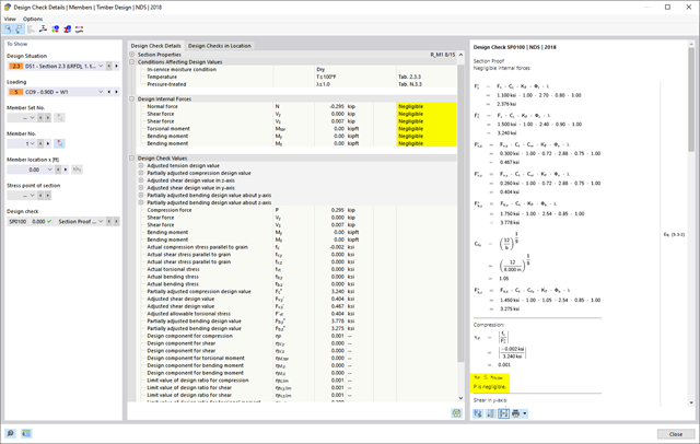
- Design of tension, compression, bending, shear, torsion, and combined internal forces
- Consideration of a notch
- Design of compression perpendicular to the grain on the end and intermediate supports with (EC 5) and without reinforcement elements (fully threaded screws)
- Optional shear force reduction at the support (see the Product Feature)
- Design of curved and tapered members
- Consideration of higher strengths for similar components that are close together (factor ksys according to EN 1995‑1‑1, 6.6(1)-(3))
- Option to increase shear resistance for softwood timber according to DIN EN 1995‑1‑1:NA NDP to 6.1.7(2)
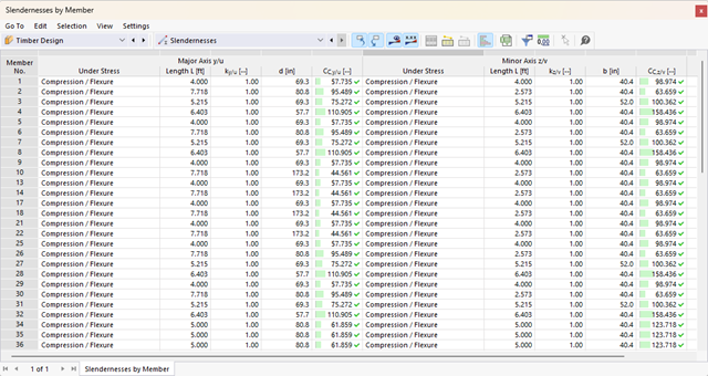
- Stability analyses for flexural buckling, torsional buckling, and flexural-torsional buckling under compression
- Import of the effective lengths from the calculation using the Structure Stability add-on
- Graphical input and check of the defined nodal supports and effective lengths for stability analysis
- Determination of the equivalent member lengths for tapered members
- Consideration of Lateral-Torsional Bracing Position
- Lateral-torsional buckling analysis of the structural components subjected to moment loading
- Depending on the standard, a choice between user-defined input of Mcr, analytical method from the standard, and use of internal eigenvalue solver
- Consideration of a shear panel and a rotational restraint when using the eigenvalue solver
- Graphical display of a mode shape if the eigenvalue solver was used
- Stability analysis of structural components with the combined compression and bending stress, depending on the design standard
- Comprehensible calculation of all necessary coefficients, such as the factors for considering moment distribution or interaction factors
- Alternative consideration of all effects for the stability analysis when determining internal forces in RFEM/RSTAB (second-order analysis, imperfections, stiffness reduction, possibly in combination with the Torsional Warping (7 DOF) add-on)
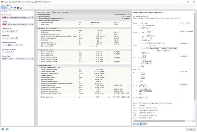
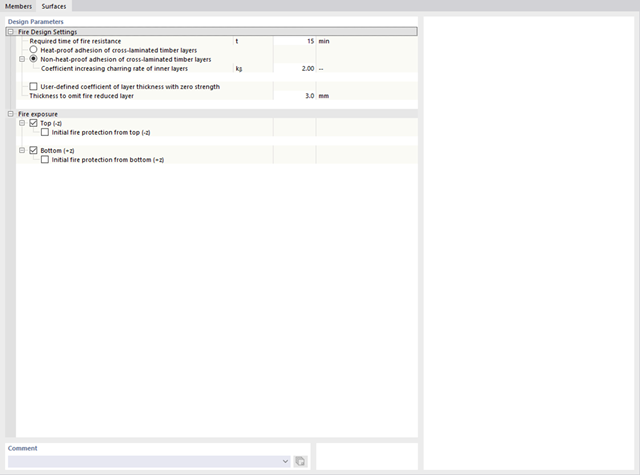
- Arbitrary definition of the charring time
- Option to calculate with or without adhesion of the layer for surface structures (cross-laminated timber)
- Free user-defined specification of the fire parameters
- Consideration of Different Effective Lengths in Fire Resistance Design
- Optional design "Compression perpendicular to grain"
- Graphical result display integrated in RFEM/RSTAB, such as a design ratio
- Complete integration of the results into the RFEM/RSTAB printout report
RFEM/RSTAB also provides a range of functions for the case of a fire. The program allows for the automatic generation of load and result combinations for the accidental design situation of fire design. The members to be designed with the corresponding internal forces are imported directly from RFEM/RSTAB. Also, all information about the material and cross-section is stored. You don't need to do anything else.
You only define the parameters relevant for the fire resistance design by assigning a fire resistance configuration to the members and surfaces to be designed. Moreover, you can also make further detailed settings, such as the definition of the fire exposure on one side up to all sides.
As you probably know, the design checks for the selected members are carried out, taking into account the defined charring time. All necessary reduction factors and coefficients are stored accordingly in the program and are taken into account when determining the load-bearing capacity. That saves you a lot of work.
The effective lengths for the equivalent member design are taken directly from the strength entries. You do not have to enter them again.
After completing the design, the program presents the fire resistance design checks clearly and with all result details. This allows you to follow the results completely transparently. The results also contain all the required parameters, so you can determine the component temperature at the design time.
In addition to all these features, the program allows you to integrate all result tables and graphics, including the ultimate and serviceability limit state results,into the global printout report of RFEM/RSTAB as a part of the steel design results.
For the design according to Eurocode 5, the parameters of the National Annexes (NA) are integrated for the following countries:
-
 DIN EN 1995-1-1/NA:2014-07 (Germany)
 -
 ÖNORM EN 1995-1-1/NA:2019-06 (Austria)
 -
 SN EN 1995-1-1/NA:2015-03 (Switzerland)
 -
 BDS EN 1995-1-1/NA:20157-06 (Bulgaria)
 -
 BS EN 1995-1-1/NA:2019-09 (United Kingdom)
 -
 CEN EN 1995-1-1/2014-05 (European Union)
 -
 CYS EN 1995-1-1/NA:2019-06 (Cyprus)
 -
 CZE EN 1995-1-1/NA:2015-05 (Czech Republic)
 -
 DS EN 1995-1-1/NA:2019-09 (Denmark)
 -
 ELOT EN 1995-1-1/NA:2010-01 (Greece)
 -
 EVS EN 1995-1-1/NA:2015-11 (Estonia)
 -
 HRN EN 1995-1-1/NA:2015-03 (Croatia)
 -
 I S. EN 1995-1-1/NA:2014-05 (Ireland)
 -
 ILNAS EN 1995-1-1/NA:2020-3 (Luxembourg)
 -
 IST EN 1995-1-1/NA:2014-09 (Iceland)
 -
 LST EN 1995-1-1/NA:2014-06 (Lithuania)
 -
 LVS EN 1995-1-1/NA:2014-12 (Latvia)
 -
 MSZ EN 1995-1-1/NA:2015-06 (Hungary)
 -
 NBN EN 1995-1-1/NA:2014-06 (Belgium)
 -
 NEN EN 1995-1-1/NA:2014-06 (Netherlands)
 -
 NF EN 1995-1-1/NA:2020-04 (France)
 -
 NP EN 1995-1-1/NA:2014-09 (Portugal)
 -
 NS EN 1995-1-1/NA:2014-08 (Norway)
 -
 PN EN 1995-1-1/NA:2014-07 (Poland)
 -
 SFS EN 1995-1-1/NA:2016-12 (Finland)
 -
 SIST EN 1995-1-1/NA:2018-01 (Slovenia)
 -
 SR EN 1995-1-1/NA:2014-12 (Romania)
 -
 SS EN 1995-1-1/NA:2018-02 (Singapore)
 -
 SS EN 1995-1-1/NA:2014-05 (Sweden)
 -
 STN EN 1995-1-1/NA:2019-12 (Slovakia)
 -
 TKP EN 1995-1-1/NA:2019-09 (Belarus)
 -
 UNE EN 1995-1-1/NA:2016-04 (Spain)
 -
 UNI EN 1995-1-1/NA:2016-11 (Italy)