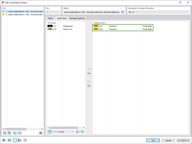
The combination wizard provides you with the option to consider more than one initial state. RFEM and RSTAB allow you to specify different initial states (prestress, form-finding, strain, and so on) for the target combinations in the combinatorics.
You can thus, for example, generate load states on the basis of a form-finding analysis with varying imperfections.
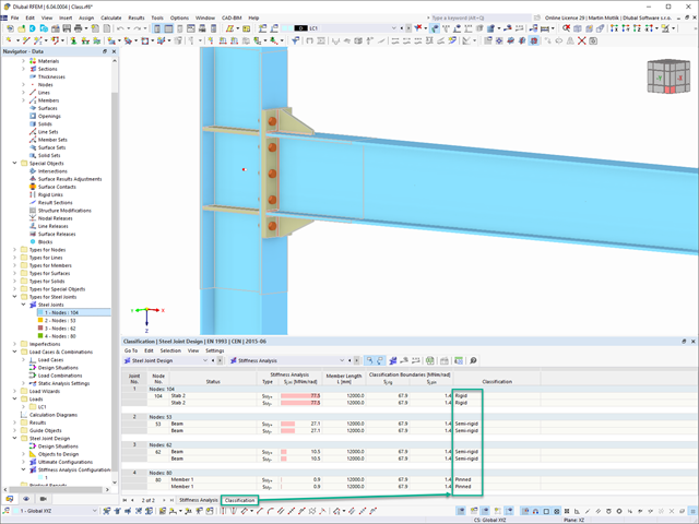
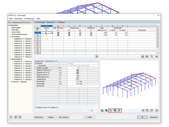
In the Steel Joints add-on, you can classify the joint stiffness.
In addition to the initial stiffness, the table also shows the limit values for hinged and rigid connections for the selected internal forces N, My, and/or Mz. The resulting classification is then displayed in tables as "hinged", "semi-rigid", or "rigid".
Go to Explanatory Video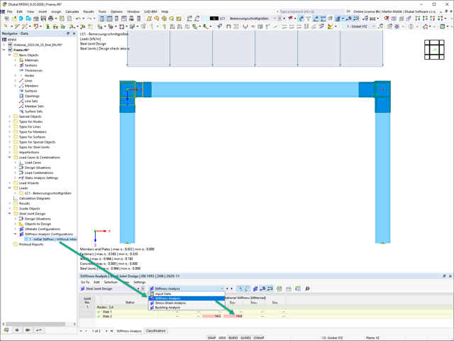
The initial stiffness Sj,ini is a crucial parameter for evaluating whether a connection can be characterized as rigid, semi-rigid, or pinned.
In the "Steel Joints" add-on, you can calculate the initial stiffness Sj,ini according to Eurocode (EN 1993‑1‑8, Section 5.2.2) and AISC (AISC 360-16, Cl. E3.4) with regard to the internal forces N, My, and/or Mz.
The optional automatic transfer of initial stiffnesses allows for a directly transfer as member hinge stiffnesses in RFEM. The entire structure is then recalculated and the resulting internal forces are automatically adopted as loads in the analysis and design of the connection models.
This automated iteration process eliminates the need for manual export and import of data, reducing the amount of work and minimizing potential sources of error.
Explanatory Video: Calculation of Initial Stiffness Sj,ini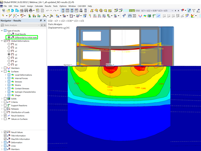
Did you already know? For load combinations, you can optionally display the difference results to the initial state. For example, you have the option for a geotechnical analysis to output the settlement as a difference to the initial state "soil self-weight".
- Calculation of deflections and comparison with the normative or manually adjusted limit values
- Consideration of a precamber for the deflection analysis
- Different limit values are possible, depending on the design situation type
- Manual Adjustment of Reference Lengths and Segmentation by Direction
- Calculation of deflections related to the initial structure or to the deformed structure
- Further detailed design checks depending on the selected design standard (for example, vibration design according to EN 1999‑1‑1, 7.2.3)
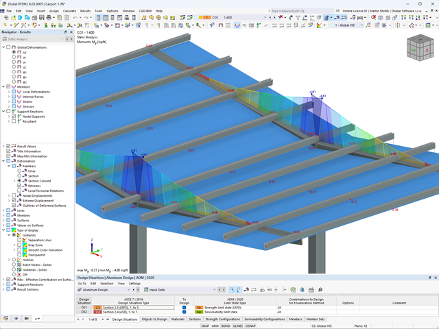
- Graphical result display integrated in RFEM/RSTAB; for example, the design ratio of a limit value, or the deformation or the sag
- Complete integration of the results into the RFEM/RSTAB printout report
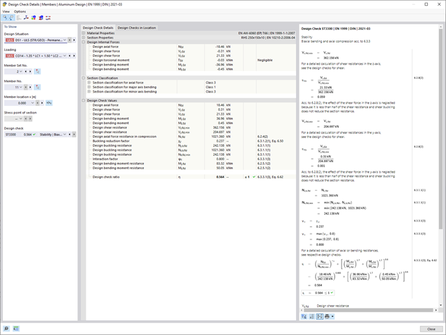
Do you prefer it clear? So do we! That's why all performed design checks for the design standard are displayed for you in a clear way. You determine a design criterion for each design check. You get design details, which include the initial values, intermediate results, and final results, arranged in a structured way for each design check. You can find the calculation process with the applied formulas, standard sources, and results in great detail in an information window in the design details.

When defining the input data for the modal analysis load case, you can consider a load case whose stiffnesses represent the initial position for the modal analysis. How do you do that? As shown in the image, select the "Consider initial state from" option. Now, open the "Initial State Settings" dialog box and define the type Stiffness as the initial state. In this load case, as of which is the initial state taken into account, you can consider the stiffness of the structural system when the tension members fail. The purpose of all of this: The stiffness from this load case is considered in the modal analysis. Thus, you obtain a clearly flexible system.

You can already see it in the image: Imperfections can also be taken into account when defining a modal analysis load case. The imperfection types that you can use in the modal analysis are notional loads from load case, initial sway via table, static deformation, buckling mode, dynamic mode shape, and group of imperfection cases.
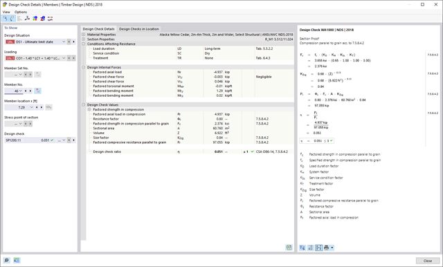
Dlubal Software just makes everything a little easier. The performed design checks of the design standard are displayed in a clear way. A design criterion is determined for each design check. Furthermore, the program deliver the design details displayed in a structured way, including the initial values, the intermediate results, and the final results. An information window in the design details shows you the calculation process with the applied formulas, standard sources, and results in great detail.
- Calculation of deflections and comparison with the normative or manually adjusted limit values
- Consideration of a precamber for the deflection analysis
- Different limit values are possible, depending on the design situation type
- Manual adjustment of reference lengths and segmentation by direction
- Calculation of deflections related to the initial structure or to the deformed structure
- Automatic consideration of time-dependent deformations by increasing the load with the creep factor (can also be user-defined on the stiffness side)
- Simplified vibration design
- Graphical result display integrated in RFEM/RSTAB; for example, the design ratio of a limit value, the deformation, or the sag
- Complete integration of the results into the RFEM/RSTAB printout report
- Calculation of deflections and comparison with the normative or manually adjusted limit values
- Consideration of a precamber for the deflection analysis
- Different limit values are possible, depending on the design situation type
- Manual adjustment of reference lengths and segmentation by direction
- Calculation of deflections related to the initial structure or to the deformed structure
- Further detailed design checks depending on the selected design standard (for example, limitation of web breathing according to EN 1993‑2)
- Graphical result display integrated in RFEM/RSTAB; for example, the design ratio of a limit value, the deformation, or the sag
- Complete integration of the results into the RFEM/RSTAB printout report
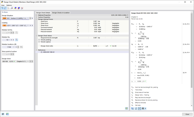
Is a clear arrangement important for you? The program provides you with a clear overview of all performed design checks for the design standard. For each design check, it is necessary to determine a design criterion. There are also design details arranged in a structured way, including the initial values, intermediate results, and final results. You can laso find here an information window where the calculation process with the applied formulas, standard sources, and results is displayed in great detail.
The structural analysis program provides you with a clear overview of all performed design checks for the design standard. You have to determine a design criterion for each design check. In addition to the ultimate limit state and the serviceability limit state design, the program checks the design rules of the standard. For each design check, there are the design details including the initial values, intermediate results, and final results, arranged in a structured way. An information window in the design details shows you the calculation process with the applied formulas, standard sources, and results in great detail.
- Calculation of transient incompressible turbulent wind flow with the BlueDyMSolver solver
- LES SpalartAllmarasDDES turbulence model
- Consideration of stationary solution as initial state for transient calculation
- Automatic determination of analysis period and time steps
- Use of intermediate results during the calculation
- Organized display of time-varying results via time step units
- Diagram of drag force and point probe results over analysis time
- Display of line probe results for any time steps in a diagram
- Freely adjustable wind permeability for surfaces (Go to Product Feature)
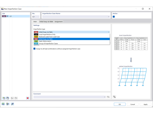
The organization of imperfections is efficiently solved by imperfection cases. The cases allow you to describe an imperfection from local imperfections, equivalent loads, initial sway via table (new), a static deformation, a buckling mode, a dynamic mode shape, or a combination of all these types (new).
Go to Explanatory Video
Compared to the RF-FORM-FINDING add-on module (RFEM 5), the following new features have been added to the Form-Finding add-on for RFEM 6:
- Specification of all form-finding load boundary conditions in one load case
- Storage of form-finding results as initial state for further model analysis
- Automatic assignment of the form-finding initial state via combination wizards to all load situations of a design situation
- Additional form-finding geometry boundary conditions for members (unstressed length, maximum vertical sag, low-point vertical sag)
- Additional form-finding load boundary conditions for members (maximum force in member, minimum force in member, horizontal tension component, tension at i-end, tension at j-end, minimum tension at i-end, minimum tension at j-end)
- Material types "Fabric" and "Foil" in material library
- Parallel form-findings in one model
- Simulation of sequentially building form-finding states in connection with the Construction Stages Analysis (CSA) add-on
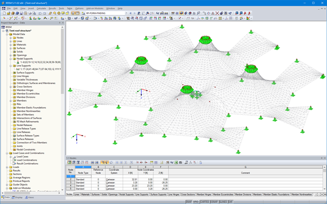
Do you know exactly how the form-finding is performed? First, the form-finding process of the load cases with the load case category "Prestress" shifts the initial mesh geometry to an optimally balanced position by means of iterative calculation loops. For this task, the program uses the Updated Reference Strategy (URS) method by Prof. Bletzinger and Prof. Ramm. This technology is characterized by equilibrium shapes that, after the calculation, comply almost exactly with the initially specified form-finding boundary conditions (sag, force, and prestress).
In addition to the pure description of the expected forces or sags on the elements to be formed, the integral approach of the URS also enables a consideration of regular forces. In the overall process, this allows, for example, for a description of the self-weight or a pneumatic pressure by means of corresponding element loads.
All these options give the calculation kernel the potential to calculate anticlastic and synclastic forms that are in an equilibrium of forces for planar or rotationally symmetric geometries. In order to be able to realistically implement both types individually or together in one environment, the calculation provide you with two ways to describe the form-finding force vectors:
- Tension method - description of the form-finding force vectors in space for planar geometries
- Projection method - description of the form-finding force vectors on a projection plane with fixation of the horizontal position for conical geometries

The form-finding process gives you a structural model with active forces in the "prestress load case" This load case shows the displacement from the initial input position to the form-found geometry in the deformation results. In the force or stress-based results (member and surface internal forces, solid stresses, gas pressures, and so on), it clarifies the state for maintaining the found form. For the analysis of the shape geometry, the program offers you a two-dimensional contour line plot with the output of the absolute height and an inclination plot for the visualization of the slope situation.
Now, a further calculation and structural analysis of the entire model is performed. For this purpose, the program transfers the form-found geometry including the element-wise strains into a universally applicable initial state. You can now use it in the load cases and load combinations.

- Automatic consideration of masses from self-weight
- Direct import of masses from load cases or load combinations
- Optional definition of additional masses (nodal, linear, or surface masses, as well as inertia masses) directly in the load cases
- Optional neglect of masses (for example, mass of foundations)
- Combination of masses in different load cases and load combinations
- Preset combination coefficients for various standards (EC 8, SIA 261, ASCE 7,...)
- Optional import of initial states (for example, to consider prestress and imperfection)
- Structure Modification
- Consideration of failed supports or members/surfaces/solids
- Definition of several modal analyses (for example, to analyze different masses or stiffness modifications)
- Selection of mass matrix type (diagonal matrix, consistent matrix, unit matrix), including user-defined specification of translational and rotational degrees of freedom
- Methods for determining the number of mode shapes (user-defined, automatic - to reach effective modal mass factors, automatic - to reach the maximum natural frequency - only available in RSTAB)
- Determination of mode shapes and masses in nodes or FE mesh points
- Results of eigenvalue, angular frequency, natural frequency, and period
- Output of modal masses, effective modal masses, modal mass factors, and participation factors
- Masses in mesh points displayed in tables and graphics
- Visualization and animation of mode shapes
- Various scaling options for mode shapes
- Documentation of numerical and graphical results in printout report

- Calculation of models consisting of member, shell, and solid elements
- Nonlinear stability analysis
- Optional consideration of axial forces from initial prestress
- Four equation solvers for an efficient calculation of various structural models
- Optional consideration of stiffness modifications in RFEM/RSTAB
- Determination of a stability mode greater than the user-defined load increment factor (Shift method)
- Optional determination of the mode shapes of unstable models (to identify the cause of instability)
- Visualization of the stability mode
- Basis for determining imperfection
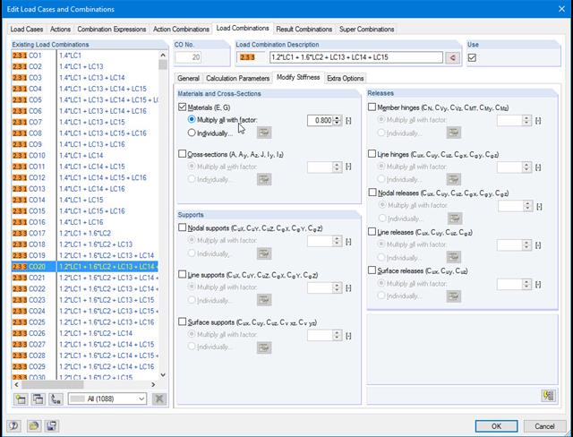
Do not lose track of stiffnesses and initial deformations. In the individual load cases or combinations, you have the option to modify the stiffnesses of materials, cross-sections, nodal, line and surface supports, and member and line hinges for all or selected members. You can also consider initial deformations from other load cases or load combinations.
.png?mw=640&hash=8cfd0c4bd093c03de543d147ffbf6f5c9250634a)
- User-defined time diagrams as a function of time, in tabular form, or as harmonic loads
- Combination of the time diagrams with RFEM/RSTAB load cases or combinations (enables definition of nodal, member, and surface loads, as well as free and generated loads varying over time)
- Combination of several independent excitation functions
- Nonlinear time history analysis with the implicit Newmark analysis (RFEM only) or the explicit analysis
- Structural damping using Rayleigh damping coefficients or Lehr's damping
- Direct import of initial deformations from a load case or combination (RFEM only)
- Stiffness modifications as initial conditions; for example, axial force effect, deactivated members (RSTAB only)
- Graphical display of results in a time history diagram
- Export of results in user-defined time steps or as an envelope
The results of the form‑finding process are a new shape and corresponding inner forces. The usual results, such as deformations, forces, stresses, and others can be displayed in the RF‑FORM‑FINDING case.
This prestressed shape is available as the initial state for all other load cases and combinations in the structural analysis.
For more ease when defining load cases, the NURBS transformation can be used (Calculation Parameters/Form-Finding). This feature moves the original surfaces and cables into position after form‑finding.
By using the grid points of surfaces or the definition nodes of NURBS surfaces, free loads can be situated on selected parts of the structure.
In the individual load cases or combinations, there is the option to modify the stiffnesses of materials; cross-sections; nodal, line and surface supports; and member and line hinges for all or selected members. Furthermore, it is possible to consider initial deformations from other load cases or load combinations.
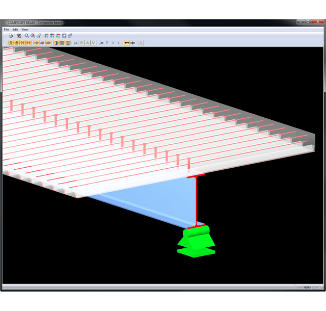
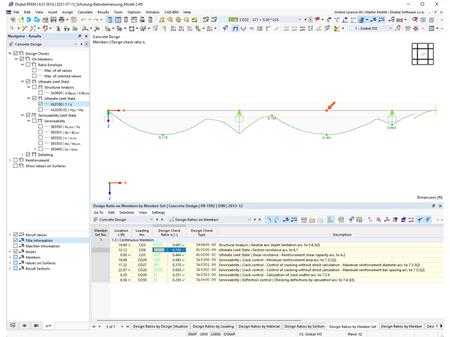
Results are displayed in result tables sorted by required designs. Clear arrangement of the results allows for easy orientation and evaluation.
Ultimate Limit State Design:
- Bending and shear force resistance with interaction
- Partial shear connecting of ductile and non-ductile connecting elements
- Determination of required shear connectors and their distribution
- Design of longitudinal shear force resistance
- Design of connection with shear connectors and of connector perimeter
- Results of governing support reactions for construction and composite stage, including loads of construction supports
- Lateral-torsional buckling analysis (for continuous beams and cantilevered girders)
- Check of cross-section classes as well as of plastic and elastic cross-section properties
Serviceability limit state design:
- Deflection Analysis
- Deformations and initial pre-cambering determined with ideal cross-section properties from creep and shrinkage
- Analysis of natural frequencies
- Crack width analysis
- Determination of support forces
All data are documented in a clearly arranged printout report, including graphics. In case of any modification, the printout report is updated automatically. COMPOSITE-BEAM is a stand-alone program and does not require the RSTAB license.
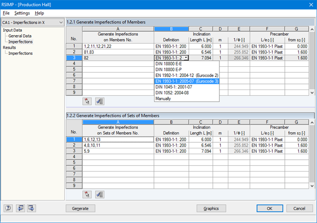
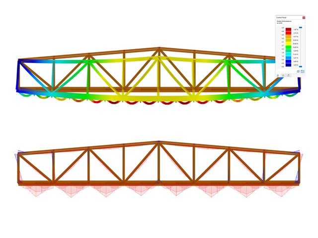
The add-on module evaluates the pre-deformation of a load case as well as mode shapes of stability or dynamic analysis. Based on this initial deformation, it is possible either to pre-deform the structure or to create a load case with equivalent imperfections of members.
The pre-deformed initial model is useful especially for structures consisting of surface and solid elements (RFEM) as well as members. It is necessary to specify only the maximum value to which the deformation is to be scaled. All FE or model nodes will be scaled with regard to the initial deformation.
Equivalent imperfections are particularly useful for beam structures. You can define inclinations and precambers of members and sets of members in the additional window. They can be generated automatically, according to standards, or defined manually. The following standards are available:
-
 EN 1992:2004
 -
EN 1993:2005
-
 DIN 18800:1990-11
 -
DIN 1045-1:2001-07
-
DIN 1052:2004-08
Only the imperfection resulting from the initial deformation on the relevant member is applied. In addition, you can consider the reduction factors. This way, it is possible to apply the imperfection efficiently.
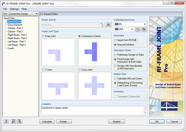
- Design of knee joints, T-joints, cross joints, and continuous column connections with I-shaped sections
- Import of geometry and load data from RFEM/RSTAB or manual specification of the connection (for example, for recalculation without an existing RFEM/RSTAB model)
- Flush top connections or connections with bolt row in extension
- Design of positive and negative frame joint moments
- Various inclinations of right and left horizontal beams as well as application to frames of duopitch and monopitch roofs
- Consideration of additional flanges in a horizontal beam, for example for tapered sections
- Symmetrical and asymmetrical T-joints or cross joints
- Two-sided connection with different cross-section depth on the right and left
- Automatic preliminary design of bolt layout and required stiffening
- Optional design mode with possibility to specify all bolt spacing, welds, and sheet thicknesses
- Screwability check with adjustable dimensions of used wrenches
- Connection classification by stiffness and calculation of the spring stiffness of connections considered in the internal forces determination
- Check up to 45 individual designs (components) of the connection
- Automatic determination of governing internal forces for each individual design
- Controllable connection graphics in rendering mode with specifications of material, sheet thickness, welds, bolt spacing, and all dimensions for construction
- Integrated and flexibly extensible settings of National Annexes according to EN 1993-1-8 standard
- Automatic conversion of internal forces from structural analysis into respective sections, also for eccentric member connections
- Automatic determination of initial stiffness Sj,ini of the connection
- Detailed plausibility check of all dimensions, including specifications of input limits (for example, for edge distances and hole spacing)
- Optional application of compression forces to a column through contact
- Possibility to update the cross-section depth of horizontal beams in case of tapered connections after connection geometry optimization in RF-/FRAME-JOINT Pro
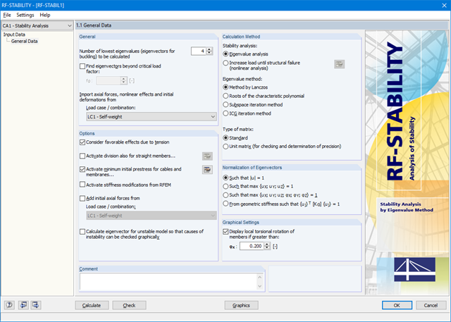
First of all, it is necessary to select a load case or combination whose axial forces are to be used in the stability analysis. It is possible to define another load case to, for example, For example, you have to consider an initial prestress.
Then, you can select the linear or non-linear analysis to be performed. Depending on the application, you can use a direct calculation method, such as according to Lanczos or the ICG iteration method. Members not integrated in surfaces are usually displayed as member elements with two FE nodes. It is not possible to determine the local buckling of single members on these elements. Therefore, you have the option to divide members automatically.

If there is a load case or load combination in the program, the stability calculation is activated. You can define another load case in order to consider initial prestress, for example.
For this, you need to specify whether to perform a linear or nonlinear analysis. Depending on the case of application, you can select a direct calculation method, such as the Lanczos method or the ICG iteration method. Members not integrated in surfaces are usually displayed as member elements with two FE nodes. With such elements, the program cannot determine the local buckling of single members. That's why you have the option to divide members automatically.
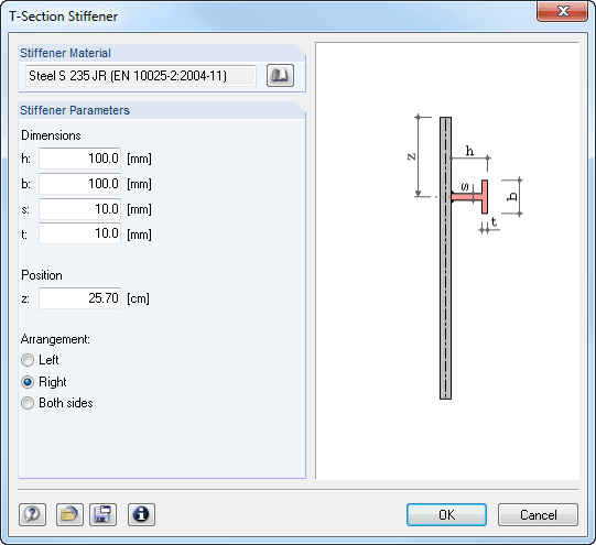
Initially, it is necessary to define material data, panel dimensions, and boundary conditions (hinged, built-in, unsupported, hinged-elastic). It is possible to transfer the data from RFEM/RSTAB. Then, boundary stresses can be either defined for each load case manually or imported from RFEM/RSTAB.
Stiffeners are modeled as spatially effective surface elements that are eccentrically connected to the plate. Therefore, it is not necessary to consider the stiffener eccentricities by effective widths. The bending, shear, strain, and St. Venant stiffness of stiffeners as well as the Bredt stiffness of closed stiffeners is determined automatically in a 3D model.