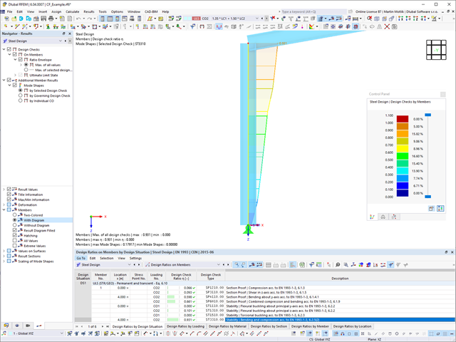
68 Wyniki
Wyświetl wyniki:
Sortuj według:
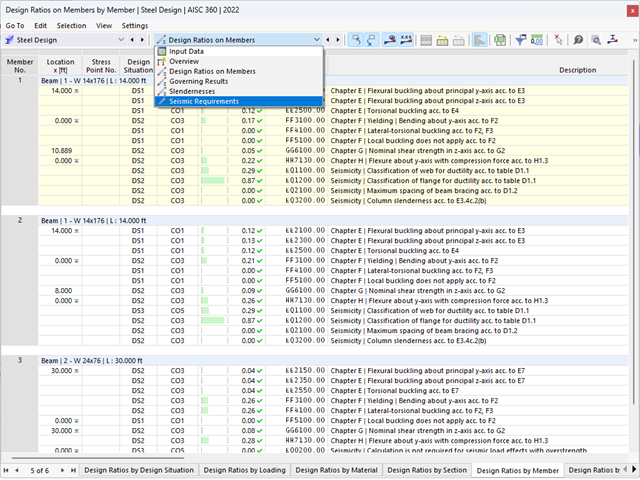
Wynik obliczeń sejsmicznych jest podzielony na dwie sekcje: wymagania dotyczące prętów i połączeń.
"Wymagania sejsmiczne" zawierają Wymaganą wytrzymałość na zginanie i Wymaganą wytrzymałość na ścinanie połączenia belka-słup dla ram sprężystych. Są one wyszczególnione w zakładce 'Połączenia ram momentowych według prętów'. W przypadku ram stężonych w zakładce 'Połączenie stężone według pręta' podawana jest Wymagana wytrzymałość połączenia na rozciąganie oraz Wymagana wytrzymałość połączenia na ściskanie stężeń.
Przeprowadzone kontrole obliczeń są przedstawiane w tabelach. W szczegółach kontroli obliczeń w przejrzysty sposób przedstawione są wzory i odniesienia do normy.
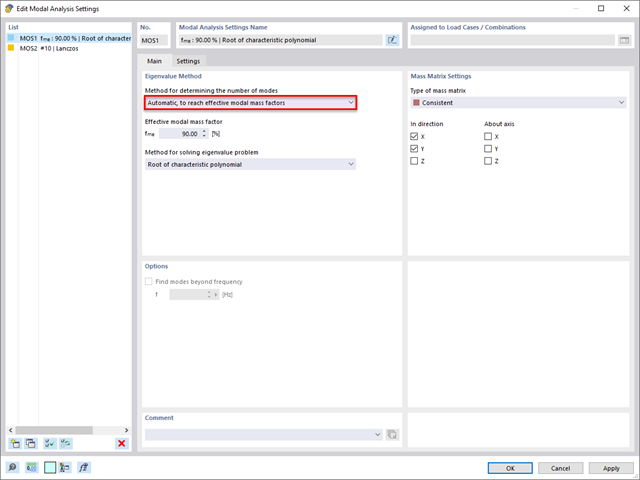
Rozszerzenie Analiza modalna umożliwia automatyczne zwiększanie poszukiwanych wartości własnych do momentu osiągnięcia zdefiniowanego współczynnika efektywnej masy modalnej. Uwzględniane są wszystkie kierunki translacyjne, które zostały aktywowane jako masy do analizy modalnej.
W ten sposób można łatwo obliczyć wymagane 90% efektywnej masy modalnej dla metody spektrum odpowiedzi.
- 002733
- Ogólne informacje
- Projektowanie konstrukcji stalowych RFEM 6
- Projektowanie konstrukcji stalowych RSTAB 9
Rozszerzenie Projektowanie konstrukcji stalowych umożliwia przeprowadzanie obliczeń sejsmicznych prętów stalowych zgodnie z AISC 341-16.
W tym celu dostępnych jest pięć typów systemów SFRS (Seismic Force-Resisting Systems).

W przypadku analizy spektrum odpowiedzi modeli budynków można wyświetlić współczynniki wrażliwości dla kierunków poziomych według kondygnacji.
Dzięki tym kluczowym wartościom można zinterpretować wrażliwość na efekty stateczności.
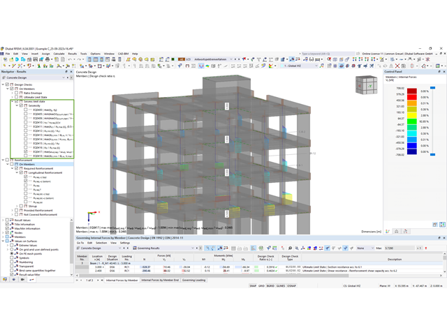
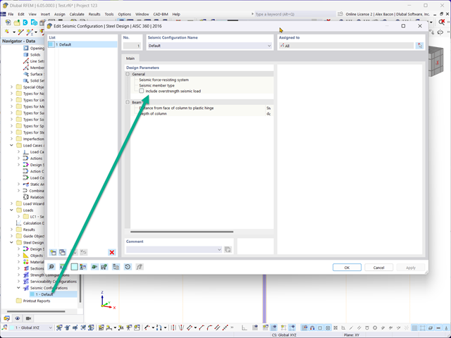
W rozszerzeniu Projektowanie konstrukcji betonowych można przeprowadzać obliczenia sejsmiczne dla prętów żelbetowych zgodnie z EC 8. Są to między innymi następujące funkcje:
- Konfiguracje obliczeń sejsmicznych
- Rozróżnianie klas ciągliwości DCL, DCM, DCH
- Możliwość przeniesienia współczynnika odpowiedzi z analizy dynamicznej
- Sprawdzenie wartości granicznej współczynnika odpowiedzi
- Weryfikacja nośności dla "Wytrzymały słup - słaba belka"
- Uszczegółowienie i reguły szczególne dla współczynnika ciągliwości krzywizny
- Uszczegółowienie i reguły szczególne dla ciągliwości lokalnej
W rozszerzeniu Projektowanie konstrukcji stalowych można przeprowadzić kontrolę obliczeń stateczności i przekrojów profili formowanych na zimno według EN 1993-1-3, zgodnie z punktami 6.1.2 - 6.1.5 i 6.1.8 - 6.1.10.
Przejdź do filmu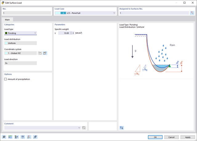
Wprowadzenie typu obciążenia Woda stojąca umożliwia symulację oddziaływań deszczu na powierzchnie wielokrotnie zakrzywione, z uwzględnieniem przemieszczeń według analizy dużych odkształceń.
Ten numeryczny proces analizy deszczowej analizuje przypisaną geometrię powierzchni i określa, które składowe wody deszczowej spływają, a które gromadzą się w postaci kałuży (kieszeni wodnych) na powierzchni. Rozmiar kałuży powoduje wówczas odpowiednie obciążenie pionowe do analizy statyczno-wytrzymałościowej.
Funkcja ta jest przeznaczona do analizy w przybliżeniu poziomych geometrii dachów membranowych pod obciążeniem deszczem.
Przejdź do filmu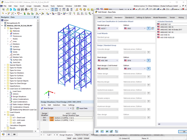
Wymiarowanie prętów stalowych formowanych na zimno zgodnie z AISI S100-16/CSA S136-16 jest dostępne w RFEM 6. Dostęp do obliczeń można uzyskać, wybierając normy „AISC 360” lub „CSA S16” w rozszerzeniu Projektowanie konstrukcji stalowych. Następnie dla obliczeń elementów formowanych na zimno automatycznie wybierane jest „AISI S100” lub „CSA S136”.
Do obliczania sprężystego obciążenia wyboczeniowego pręta program RFEM stosuje metodę DSM. Bezpośrednia metoda wytrzymałości oferuje dwa typy rozwiązań, numeryczne (metoda pasm skończonych) i analityczne (specyfikacja). Krzywą charakterystyczną (sygnaturę) FSM i kształty wyboczenia można wyświetlić w oknie dialogowym Przekroje.
- 002567
- Ogólne informacje
- Projektowanie konstrukcji stalowych RFEM 6
- Projektowanie konstrukcji stalowych RSTAB 9
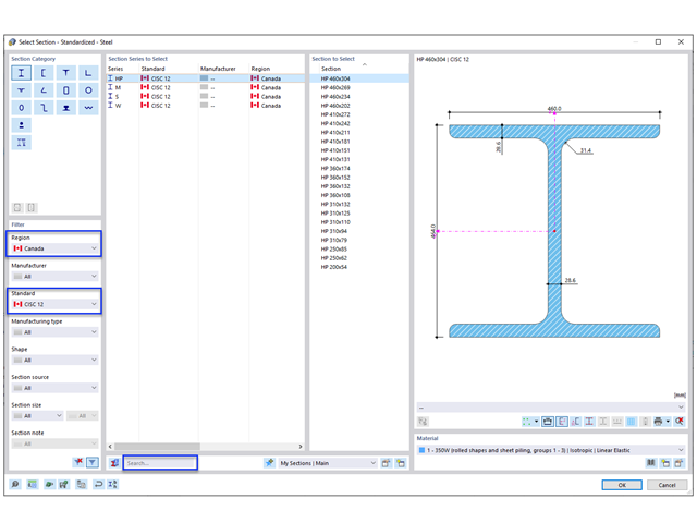
Nowe przekroje stalowe zgodnie z najnowszą instrukcją CISC (12 wydanie) są dostępne w programie RFEM 6. Przekroje są wymienione w bibliotece Znormalizowane. W filtrze należy wybrać region „Kanada”, a normę „CISC 12”. Alternatywnie nazwę przekroju można wprowadzić bezpośrednio w polu wyszukiwania znajdującym się w dolnej części okna dialogowego.
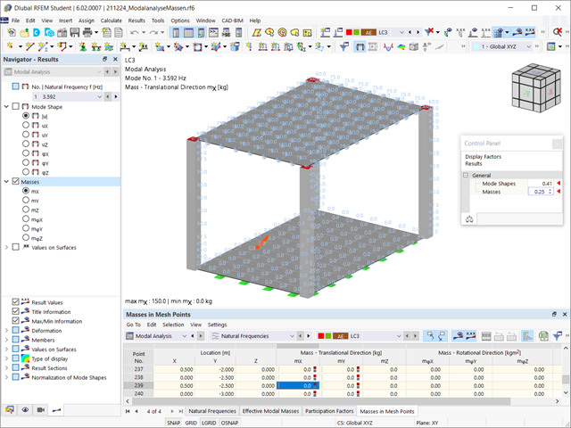
Czy odkryłeś już tabelaryczne i graficzne przedstawianie mas w punktach siatki? Po prawej, jest to również jeden z wyników analizy modalnej w programie RFEM 6. W ten sposób można sprawdzić importowane masy, które zależą od różnych ustawień analizy modalnej. Mogą być one wyświetlane w zakładce Masy w punktach siatki tabeli Wyniki. Tabela zawiera przegląd następujących wyników: Masa - kierunek przesuwny (mX, mY, mZ ), Masa - kierunek obrotowy (mφX, mφY, mφZ ) oraz suma mas. Czy nie byłoby lepiej, gdybyś jak najszybciej przeprowadził ocenę graficzną? Następnie można również wyświetlić graficznie masy w punktach siatki.
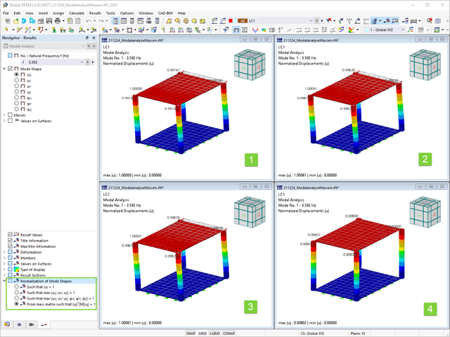
Jak już wiesz, po pomyślnym zakończeniu obliczeń wyniki przypadku obciążenia w Analizie modalnej są wyświetlane w programie. Die erste Eigenform ist für Sie also sofort grafisch oder animiert zu sehen. Dabei können Sie die Darstellung der Eigenformnormierung komfortabel anpassen. Erledigen Sie das am besten direkt im Ergebnisnavigator, wo Sie zur Visualisierung der Eigenformen eine von vier Optionen auswählen:
- Wert des Eigenformvektors uj auf 1 skalieren (berücksichtigt nur die Translationskomponenten)
- Auswahl der maximalen Translationskomponente des Eigenvektors und Einstellung auf 1
- Betrachtung der gesamten Eigenform (inklusive der Rotationskomponenten), Auswahl des Maximums und Einstellung auf 1
- Setzen der modalen Massen mi für jeden Eigenwert auf 1 kg
Ausführlichere Erläuterungen der Normierung der Eigenformen finden Sie hier: Instrukcja online .
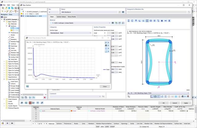
Podczas wymiarowania zgodnie z EN 1993-1-3, możliwe jest przedstawienie graficzne postaci własnej wyboczenia dystorsyjnego przekroju oraz dla przekrojów RSECTION.
Kształt postaci własnej można również wyprowadzić w RSECTION 1 dla przekrojów z biblioteki.
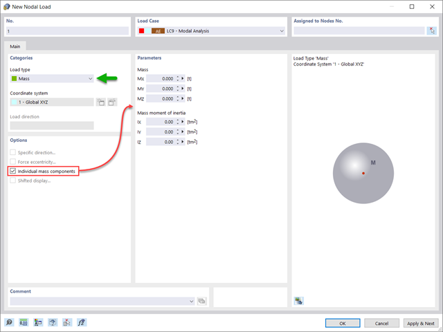
Czy oprócz obciążeń statycznych chcesz uwzględnić również inne obciążenia jako masy? Program umożliwia to dla obciążeń węzłowych, prętowych, liniowych i powierzchniowych. W tym celu podczas definiowania obciążenia należy wybrać typ Obciążenie masą. Dla takich obciążeń należy zdefiniować masę lub składowe masy w kierunkach X, Y i Z. W przypadku mas węzłowych można dodatkowo zdefiniować momenty bezwładności X, Y i Z w celu modelowania bardziej złożonych punktów mas.
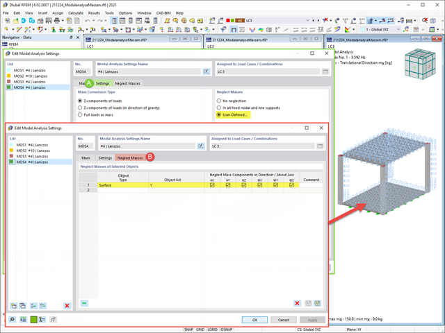
Często zachodzi potrzeba pominięcia mas. Dzieje się tak zwłaszcza w przypadku, gdy wyniki analizy modalnej mają być wykorzystane do analizy sejsmicznej. W tym celu wymagane jest 90% efektywnej masy modalnej w każdym kierunku. Pozwala to na pominięcie masy we wszystkich utwierdzonych podporach węzłowych i liniowych. Program automatycznie dezaktywuje powiązane masy.
Obiekty, których masy mają zostać pominięte w analizie modalnej, można również wybrać ręcznie. Dla lepszego widoku pokazaliśmy to ostatnie na rysunku. W wyniku wyboru przez użytkownika obiektów masowych wraz z skojarzonymi z nimi składowymi masowymi można pominąć masy.
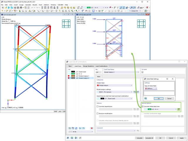
Podczas definiowania danych wejściowych dla przypadku obciążenia analizy modalnej można uwzględnić przypadek obciążenia, którego sztywności reprezentują początkową pozycję analizy modalnej. Jak to zrobić? Jak pokazano na rysunku, należy wybrać opcję "Uwzględnij stan początkowy z". Teraz otwórz okno dialogowe "Ustawienia stanu początkowego" i zdefiniuj typ Sztywność jako stan początkowy. W tym przypadku obciążenia, który jest stanem początkowym branym pod uwagę, można uwzględnić sztywność układu konstrukcyjnego, gdy pręty rozciągane ulegają uszkodzeniu. Celem tego wszystkiego: Sztywność z tego przypadku obciążenia jest uwzględniana w analizie modalnej. W ten sposób uzyskuje się wyraźnie elastyczny system.
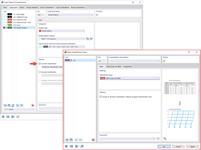
Widać to już na obrazku: Imperfekcje można również uwzględnić podczas definiowania przypadku obciążenia w analizie modalnej. Typy imperfekcji, które mogą być stosowane w analizie modalnej, to obciążenia hipotetyczne z przypadku obciążenia, początkowe przemieszczenie w tabeli, odkształcenie statyczne, postać wyboczeniowa, postać dynamiczna oraz grupa przypadków imperfekcji.
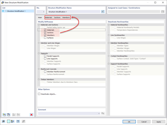
Czy wiecie, że...? W przypadkach obciążeń typu Analiza modalna można z łatwością wprowadzać zmiany konstrukcyjne. Pozwala to na przykład na indywidualne dostosowanie sztywności materiałów, przekrojów, prętów, powierzchni, przegubów i podpór. W przypadku niektórych rozszerzeń można również modyfikować sztywności. Po wybraniu obiektów ich właściwości sztywności są dostosowywane do typu obiektu. W ten sposób można je zdefiniować w osobnych zakładkach.
Czy chcesz przeanalizować uszkodzenie obiektu (na przykład słupa) w analizie modalnej? Jest to również możliwe bez żadnych problemów. Wystarczy przejść do okna Modyfikacja konstrukcji i dezaktywować odpowiednie obiekty.
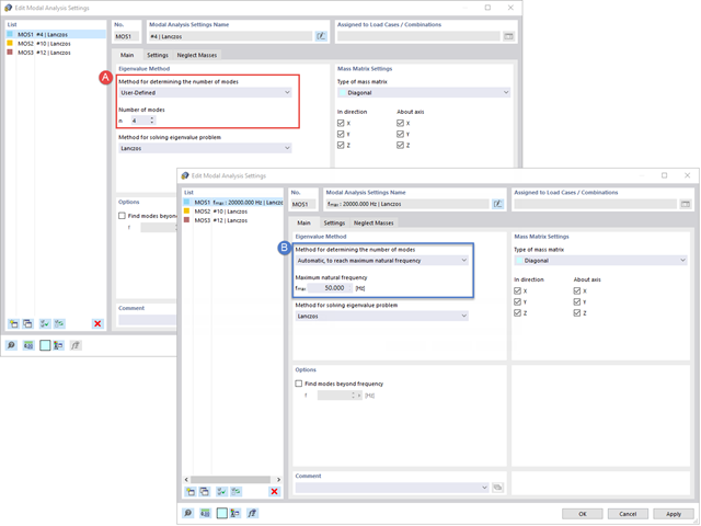
Twoim celem jest określenie liczby postaci drgań własnych? Program oferuje dwie metody. Z jednej strony, można ręcznie zdefiniować liczbę najmniejszych kształtów drgań, które mają zostać obliczone. W tym przypadku liczba dostępnych kształtów postaci zależy od stopni swobody (tzn. liczby punktów mas swobodnych pomnożonych przez liczbę kierunków, w których działają masy). Jest to jednak ograniczone do 9999. Z drugiej strony, maksymalną częstotliwość drgań własnych można ustawić w taki sposób, w jaki program określił kształty automatycznie, aż do osiągnięcia zadanej częstotliwości drgań własnych.
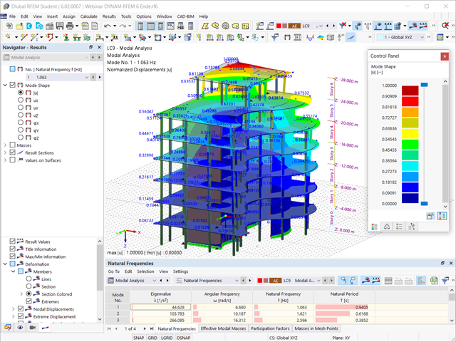
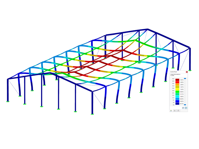
Czy obliczenia się zakończyły? Wyniki analizy modalnej są wówczas dostępne zarówno w formie graficznej, jak i tabelarycznej. Wyświetl tabele wyników dla przypadku obciążenia lub przypadków obciążeń analizy modalnej. Dzięki temu na pierwszy rzut oka można zobaczyć wartości własne, częstotliwości kątowe, częstotliwości i okresy drgań własnych konstrukcji. W przejrzysty sposób wyświetlane są również efektywne masy modalne, modalne współczynniki masy i współczynniki udziału.
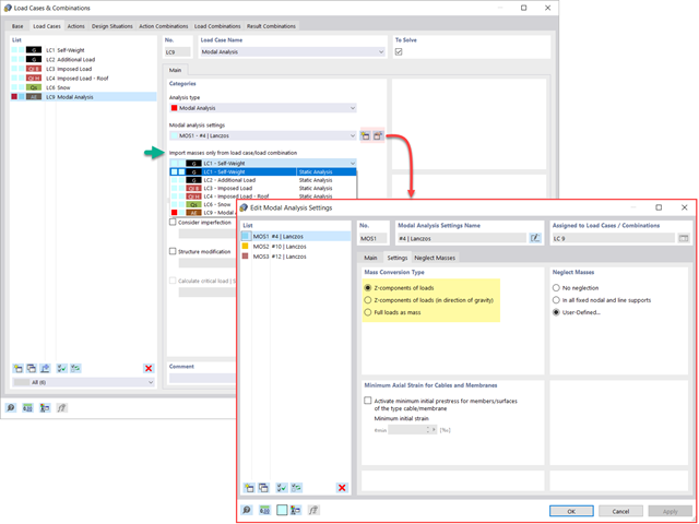
Dostępnych jest kilka opcji definiowania mas dla analizy modalnej. Masy od ciężaru własnego są uwzględniane automatycznie, natomiast obciążenia i masy można uwzględnić bezpośrednio w przypadku obciążenia typu analiza modalna. Potrzebujesz więcej opcji? Należy wybrać, czy obciążenia pełne mają być uwzględniane jako masy, składowe obciążenia w globalnym kierunku Z, czy tylko składowe obciążenia w kierunku siły ciężkości.
Program oferuje dodatkową lub alternatywną opcję importu mas: Ręczna definicja kombinacji obciążeń, począwszy od których masy są uwzględniane w analizie modalnej. Wybrałeś normę obliczeniową? Następnie można utworzyć sytuację obliczeniową typu Kombinacja mas sejsmicznych. W ten sposób program automatycznie oblicza sytuację masową dla analizy modalnej zgodnie z preferowaną normą obliczeniową. Innymi słowy: Program tworzy kombinację obciążeń na podstawie współczynników kombinacji wstępnie ustawionych dla wybranej normy. Zawiera on masy użyte do analizy modalnej.
- 002317
- Ogólne informacje
- Projektowanie konstrukcji stalowych RFEM 6
- Projektowanie konstrukcji stalowych RSTAB 9
- Obliczanie ugięć i porównanie z normatywnymi lub ręcznie dostosowanymi wartościami granicznymi
- Uwzględnienie wygięcia wstępnego w analizie ugięcia
- W zależności od typu sytuacji obliczeniowej możliwe są różne wartości graniczne
- Ręczne dostosowywanie długości odniesienia i segmentacji według kierunku
- Obliczanie ugięć w odniesieniu do konstrukcji początkowej lub do konstrukcji odkształconej
- Dalsze szczegółowe obliczenia w zależności od wybranej normy obliczeniowej (np. ograniczenie oddychania środnika zgodnie z EN 1993-2)
- Graficzne wyświetlanie wyników zintegrowane z RFEM/RSTAB; na przykład stopień wykorzystania wartości granicznej, odkształcenie lub ugięcie
- Pełna integracja wyników z protokołem wydruku programu RFEM/RSTAB
- 002318
- Ogólne informacje
- Projektowanie konstrukcji stalowych RFEM 6
- Projektowanie konstrukcji stalowych RSTAB 9
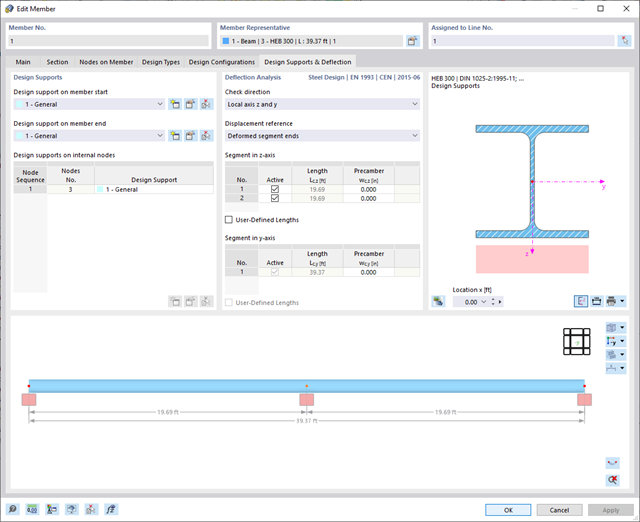
W programie RFEM/RSTAB istnieje możliwość wygenerowania, a następnie obliczenia kombinacji obciążeń lub wyników wymaganych dla stanu granicznego użytkowalności. Sytuacje obliczeniowe można wybrać do analizy ugięć w rozszerzeniu Projektowanie konstrukcji stalowych. Obliczone wartości odkształceń są odpowiednio określane w każdym miejscu pręta, w zależności od określonego wygięcia wstępnego i układu odniesienia. Na koniec można porównać te wartości odkształceń z wartościami granicznymi.
Czy wiecie, że...? Wartość graniczną deformacji można określić indywidualnie dla każdego elementu konstrukcyjnego w Konfiguracja stanu granicznego użytkowalności. Jako dopuszczalną wartość graniczną należy zdefiniować maksymalne odkształcenie w zależności od długości odniesienia. Poprzez zdefiniowanie podpór obliczeniowych można podzielić komponenty na segmenty w celu automatycznego określenia odpowiedniej długości odniesienia dla każdego kierunku obliczeń.
W zależności od położenia przydzielonych podpór obliczeniowych, rozróżnienie między belkami i wspornikami jest dokonywane automatycznie, dzięki czemu można odpowiednio określić wartość graniczną.
- 002319
- Ogólne informacje
- Projektowanie konstrukcji stalowych RFEM 6
- Projektowanie konstrukcji stalowych RSTAB 9
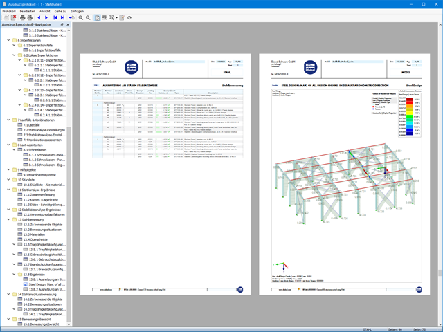
Zasady sprawdzania stanu granicznego użytkowalności można znaleźć w tabelach wyników w rozszerzeniu Projektowanie konstrukcji stalowych. Wyniki obliczeń można wyświetlić ze wszystkimi szczegółami w każdym miejscu obliczanych prętów. Ponadto dostępne są grafiki z wykresami wyników i stopni wykorzystania. Zapewnia to dobry przegląd sytuacji.
Wszystkie tabele wyników i grafiki można również zintegrować z globalnym protokołem wydruku programu RFEM/RSTAB jako część wyników wymiarowania stali. Dzięki temu można wyświetlać i dokumentować odkształcenia całej konstrukcji w ramach funkcji programu RFEM/RSTAB, niezależnie od rozszerzenia.
- 002320
- Ogólne informacje
- Projektowanie konstrukcji stalowych RFEM 6
- Projektowanie konstrukcji stalowych RSTAB 9
- Ręczne określenie temperatury krytycznej elementu lub automatyczne określenie temperatury elementu przez żądany czas
- Szeroki wybór krzywych pożaru: standardowa krzywa temperatura-czas, krzywa pożaru zewnętrznego, krzywa węglowodorów
- Ręczne dostosowywanie istotnych współczynników do określania temperatury stali
- Uwzględnienie cynkowania ogniowego elementów konstrukcyjnych przy określaniu temperatury stali
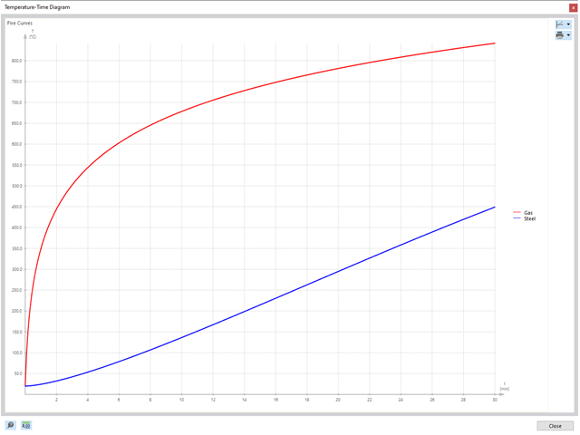
- Wyniki wykresu temperatura-czas dla temperatury gazu i stali
- Podczas określania temperatury można uwzględnić okładzinę ogniochronną w postaci obrysu lub okładziny skrzynkowej wykonanej z materiałów niezależnych od temperatury
- Wymiarowanie prętów ze stali węglowej lub nierdzewnej
- Obliczenia przekrojów i analiza stateczności (metoda prętów zastępczych) zgodnie z EN 1993-1-2, rozdz. 4.2.3
- Obliczenia przekrojów klasy 4 zgodnie z EN 1993-1-2, Załącznik E.
- 002321
- Ogólne informacje
- Projektowanie konstrukcji stalowych RFEM 6
- Projektowanie konstrukcji stalowych RSTAB 9
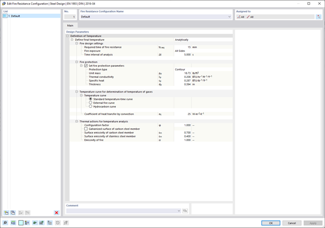
Programy do analizy statyczno-wytrzymałościowej RFEM/RSTAB oferują szereg zautomatyzowanych funkcji, które ułatwiają codzienną pracę. Jednym z nich jest automatyczne generowanie kombinacji obciążeń i wyników dla wyjątkowej sytuacji obliczeniowej w obliczeniach odporności ogniowej. Pręty, które mają zostać zwymiarowane wraz z odpowiednimi siłami wewnętrznymi, są importowane bezpośrednio z programu RFEM/RSTAB. Nie musisz'robić nic więcej. Program zachował również wszystkie informacje o materiale i przekroju.
Poprzez przypisanie konfiguracji odporności ogniowej do obliczanych prętów, użytkownik definiuje parametry istotne dla obliczeń odporności ogniowej. Tutaj można ręcznie określić krytyczną temperaturę stali w czasie projektowania. Temperaturę wyznaczaną przez program można określić automatycznie dla określonego czasu trwania pożaru. Do wyboru dostępne są różne krzywe temperatury pożaru i środki ochrony przeciwpożarowej. Można również wprowadzić dalsze szczegółowe ustawienia, takie jak zdefiniowanie ekspozycji na ogień ze wszystkich stron lub z trzech stron
- 002322
- Ogólne informacje
- Projektowanie konstrukcji stalowych RFEM 6
- Projektowanie konstrukcji stalowych RSTAB 9
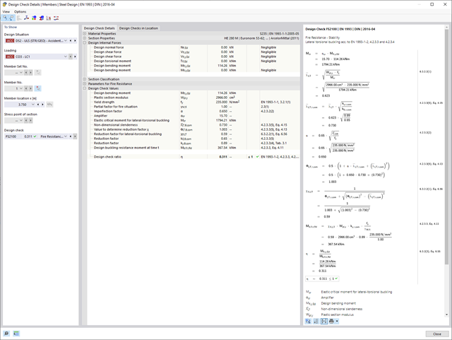
Weryfikacje wybranych prętów są przeprowadzane z uwzględnieniem decydującej temperatury elementu. W rozszerzeniu Projektowanie konstrukcji stalowych można przeprowadzić obliczenia przekrojów i analizy stateczności zgodnie z EN 1993-1-2, sekcja 4.2.3. Wszystkie niezbędne współczynniki i współczynniki redukcyjne są odpowiednio zapisywane i uwzględniane przy określaniu nośności.
Długości efektywne dla obliczeń pręta zastępczego są pobierane bezpośrednio z danych dotyczących wytrzymałości. Nie ma potrzeby'wprowadzania ich ponownie.
W każdym obliczeniu najpierw należy przeprowadzić klasyfikację przekroju. W przypadku przekrojów klasy 4 obliczenia są przeprowadzane automatycznie zgodnie z normą EN 1993-1-2, Załącznik E.
- 002323
- Ogólne informacje
- Projektowanie konstrukcji stalowych RFEM 6
- Projektowanie konstrukcji stalowych RSTAB 9
Po zakończeniu obliczeń, Dlubal Software przedstawia w przejrzysty sposób analizę odporności ogniowej wraz ze wszystkimi szczegółami wyników. Dzięki temu wyniki są zrozumiałe. Ponadto wyniki zawierają również wszystkie parametry wymagane do określenia temperatury elementu w czasie projektowania.
Rozkład temperatury w elemencie konstrukcyjnym można również ocenić za pomocą wykresu temperatura-czas.
Wszystkie tabele i grafiki wyników, w tym wyniki obliczeń stanu granicznego nośności i użytkowalności, można zintegrować z globalnym protokołem wydruku programu RFEM/RSTAB jako część wyników obliczeń konstrukcji stalowej.

- 002324
- Ogólne informacje
- Projektowanie konstrukcji stalowych RFEM 6
- Projektowanie konstrukcji stalowych RSTAB 9
W przypadku obliczeń zgodnie z Eurokodem 3 parametry załączników krajowych (NA) są zintegrowane dla następujących krajów:
-
 DIN EN 1993-1-1/NA:2020-11 (Niemcy)
 -
 ÖNORM EN 1993-1-1/NA:2015-12 (Austria)
 -
 SN EN 1993-1-1/NA:2016-07 (Szwajcaria)
 -
 BDS EN 1993-1-1/NA:2015-10 (Bułgaria)
 -
 BS EN 1993-1-1/NA:2016-07 (Wielka Brytania)
 -
 CEN EN 1993-1-1/2015-06 (Unia Europejska)
 -
 CYS EN 1993-1-1/NA:2015-07 (Cypr)
 -
 CZE EN 1993-1-1/NA:2016-06 (Republika Czeska)
 -
 DS EN 1993-1-1/NA:2015-07 (Dania)
 -
 ELOT EN 1993-1-1/NA:2017-01 (Grecja)
 -
 EVS EN 1993-1-1/NA:2015-08 (Estonia)
 -
 HRN EN 1993-1-1/NA:2016-03 (Chorwacja)
 -
 I S. EN 1993-1-1/NA:2016-03 (Irlandia)
 -
 ILNAS EN 1993-1-1/NA:2015-06 (Luksemburg)
 -
 IST EN 1993-1-1/NA:2015-11 (Islandia)
 -
 LST EN 1993-1-1/NA:2017-01 (Litwa)
 -
 LVS EN 1993-1-1/NA:2015-10 (Łotwa)
 -
 MS EN 1993-1-1/NA:2010-01 (Malezja)
 -
 MSZ EN 1993-1-1/NA:2015-11 (Węgry)
 -
 NBN EN 1993-1-1/NA:2015-07 (Belgia)
 -
 NEN EN 1993-1-1/NA:2016-12 (Holandia)
 -
 NF EN 1993-1-1/NA:2016-02 (Francja)
 -
 NP EN 1993-1-1/NA:2009-03 (Portugalia)
 -
 NS EN 1993-1-1/NA:2015-09 (Norwegia)
 -
 PN EN 1993-1-1/NA:2015-08 (Polska)
 -
 SFS EN 1993-1-1/NA:2015-08 (Finlandia)
 -
 SIST EN 1993-1-1/NA:2016-09 (Słowenia)
 -
 SR EN 1993-1-1/NA:2016-04 (Rumunia)
 -
 SS EN 1993-1-1/NA:2019-05 (Singapur)
 -
 SS EN 1993-1-1/NA:2015-06 (Szwecja)
 -
 STN EN 1993-1-1/NA:2015-10 (Słowacja)
 -
 TKP EN 1993-1-1/NA:2015-04 (Białoruś)
 -
 UNE EN 1993-1-1/NA:2016-02 (Hiszpania)
 -
 UNI EN 1993-1-1/NA:2015-08 (Włochy)
- 002325
- Ogólne informacje
- Projektowanie konstrukcji stalowych RFEM 6
- Projektowanie konstrukcji stalowych RSTAB 9
Należy przeprowadzić obliczenia odporności ogniowej ze zredukowaną nośnością na podstawie temperatury elementu, wyznaczonej automatycznie w czasie projektowania. Można to określić automatycznie na podstawie różnych krzywych temperatury w programie (standardowa krzywa temperatura-czas, krzywa pożaru zewnętrznego, krzywa węglowodorów). W przypadku innych typów określania temperatury można również ręcznie określić temperaturę, która zostanie zastosowana w obliczeniach. Można to na przykład określić zgodnie z parametryczną krzywą temperatura-czas z normy DIN EN 1991-1-2 lub z protokołu ochrony przeciwpożarowej.
- 002326
- Ogólne informacje
- Projektowanie konstrukcji stalowych RFEM 6
- Projektowanie konstrukcji stalowych RSTAB 9
Temperatura elementu, która ma być zastosowana w czasie projektowania, jest określana automatycznie. Współczynniki używane do określania temperatury można dostosowywać. Na tym etapie najlepiej jest również wybrać cynkowanie ogniowe. Zgodnie z wytyczną DASt 027 „Wyznaczanie temperatury elementów ze stali ocynkowanej ogniowo na wypadek pożaru“, stosowana jest niższa emisyjność powierzchni stalowej, aż do osiągnięcia określonej temperatury granicznej. Ogólnie rzecz biorąc, daje to niższą temperaturę, a tym samym bardziej korzystne obliczenia odporności ogniowej.