77 Wyniki
Wyświetl wyniki:
Sortuj według:
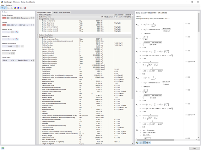
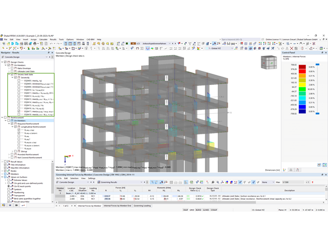
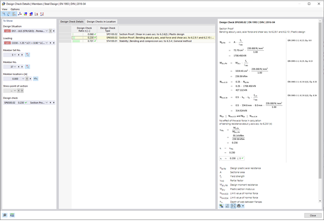
Dzięki oprogramowaniu Dlubal zawsze masz podgląd, niezależnie od tego, czy masz projekty z branży żelbetowej, stalowej, drewnianej, aluminiowej czy innej. Wzory do kontroli warunków projektowych zastosowane w obliczeniach są wyświetlane w przejrzysty sposób (wraz z odniesieniem do zastosowanego równania z normy). Te wzory do kontroli obliczeń można również uwzględnić w raporcie.
Przejdź do filmu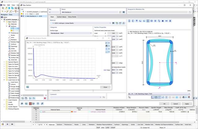
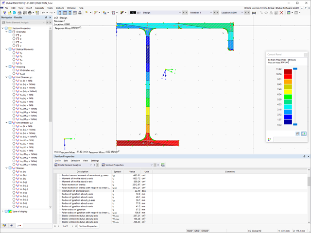
Podczas wymiarowania zgodnie z EN 1993-1-3, możliwe jest przedstawienie graficzne postaci własnej wyboczenia dystorsyjnego przekroju oraz dla przekrojów RSECTION.
Kształt postaci własnej można również wyprowadzić w RSECTION 1 dla przekrojów z biblioteki.
- 002567
- Ogólne informacje
- Projektowanie konstrukcji stalowych RFEM 6
- Projektowanie konstrukcji stalowych RSTAB 9
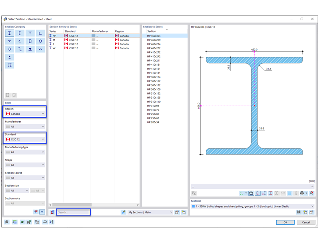
Nowe przekroje stalowe zgodnie z najnowszą instrukcją CISC (12 wydanie) są dostępne w programie RFEM 6. Przekroje są wymienione w bibliotece Znormalizowane. W filtrze należy wybrać region „Kanada”, a normę „CISC 12”. Alternatywnie nazwę przekroju można wprowadzić bezpośrednio w polu wyszukiwania znajdującym się w dolnej części okna dialogowego.
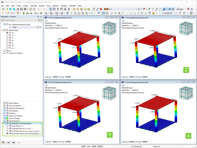
Jak już wiesz, po pomyślnym zakończeniu obliczeń wyniki przypadku obciążenia w Analizie modalnej są wyświetlane w programie. Die erste Eigenform ist für Sie also sofort grafisch oder animiert zu sehen. Dabei können Sie die Darstellung der Eigenformnormierung komfortabel anpassen. Erledigen Sie das am besten direkt im Ergebnisnavigator, wo Sie zur Visualisierung der Eigenformen eine von vier Optionen auswählen:
- Wert des Eigenformvektors uj auf 1 skalieren (berücksichtigt nur die Translationskomponenten)
- Auswahl der maximalen Translationskomponente des Eigenvektors und Einstellung auf 1
- Betrachtung der gesamten Eigenform (inklusive der Rotationskomponenten), Auswahl des Maximums und Einstellung auf 1
- Setzen der modalen Massen mi für jeden Eigenwert auf 1 kg
Ausführlichere Erläuterungen der Normierung der Eigenformen finden Sie hier: Instrukcja online .
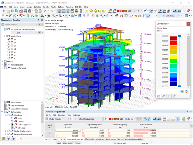
Czy obliczenia się zakończyły? Wyniki analizy modalnej są wówczas dostępne zarówno w formie graficznej, jak i tabelarycznej. Wyświetl tabele wyników dla przypadku obciążenia lub przypadków obciążeń analizy modalnej. Dzięki temu na pierwszy rzut oka można zobaczyć wartości własne, częstotliwości kątowe, częstotliwości i okresy drgań własnych konstrukcji. W przejrzysty sposób wyświetlane są również efektywne masy modalne, modalne współczynniki masy i współczynniki udziału.
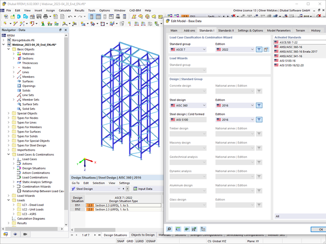
Wymiarowanie prętów stalowych formowanych na zimno zgodnie z AISI S100-16/CSA S136-16 jest dostępne w RFEM 6. Dostęp do obliczeń można uzyskać, wybierając normy „AISC 360” lub „CSA S16” w rozszerzeniu Projektowanie konstrukcji stalowych. Następnie dla obliczeń elementów formowanych na zimno automatycznie wybierane jest „AISI S100” lub „CSA S136”.
Do obliczania sprężystego obciążenia wyboczeniowego pręta program RFEM stosuje metodę DSM. Bezpośrednia metoda wytrzymałości oferuje dwa typy rozwiązań, numeryczne (metoda pasm skończonych) i analityczne (specyfikacja). Krzywą charakterystyczną (sygnaturę) FSM i kształty wyboczenia można wyświetlić w oknie dialogowym Przekroje.
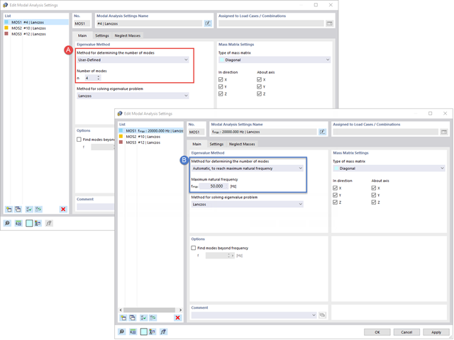
Twoim celem jest określenie liczby postaci drgań własnych? Program oferuje dwie metody. Z jednej strony, można ręcznie zdefiniować liczbę najmniejszych kształtów drgań, które mają zostać obliczone. W tym przypadku liczba dostępnych kształtów postaci zależy od stopni swobody (tzn. liczby punktów mas swobodnych pomnożonych przez liczbę kierunków, w których działają masy). Jest to jednak ograniczone do 9999. Z drugiej strony, maksymalną częstotliwość drgań własnych można ustawić w taki sposób, w jaki program określił kształty automatycznie, aż do osiągnięcia zadanej częstotliwości drgań własnych.
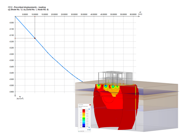
Czy jesteś gotowy na ocenę? Skorzystaj z wykresów obliczeniowych, które pokazują rozkład określonego wyniku podczas obliczeń.
Przypisanie osi pionowej i poziomej wykresu obliczeniowego można dowolnie definiować. Umożliwia to np. wyświetlenie przebiegu osiadania określonego węzła w zależności od obciążenia.
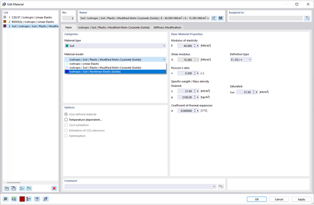
Czy chcesz modelować i analizować zachowanie bryły gruntowej? Aby to zapewnić, w programie RFEM zaimplementowano odpowiednie modele materiałowe.
Można użyć zmodyfikowanego modelu Mohra-Coulomba z liniowo-sprężystym modelem idealnie plastycznym lub nieliniowo sprężystym modelem z edometryczną relacją naprężenie-odkształcenie. Kryterium graniczne, które opisuje przejście od obszaru sprężystości do obszaru płynięcia plastycznego, jest zdefiniowane według Mohra-Coulomba.
W rozszerzeniu Projektowanie konstrukcji betonowych można przeprowadzać obliczenia sejsmiczne dla prętów żelbetowych zgodnie z EC 8. Są to między innymi następujące funkcje:
- Konfiguracje obliczeń sejsmicznych
- Rozróżnianie klas ciągliwości DCL, DCM, DCH
- Możliwość przeniesienia współczynnika odpowiedzi z analizy dynamicznej
- Sprawdzenie wartości granicznej współczynnika odpowiedzi
- Weryfikacja nośności dla "Wytrzymały słup - słaba belka"
- Uszczegółowienie i reguły szczególne dla współczynnika ciągliwości krzywizny
- Uszczegółowienie i reguły szczególne dla ciągliwości lokalnej
- 002327
- Ogólne informacje
- Projektowanie konstrukcji stalowych RFEM 6
- Projektowanie konstrukcji stalowych RSTAB 9
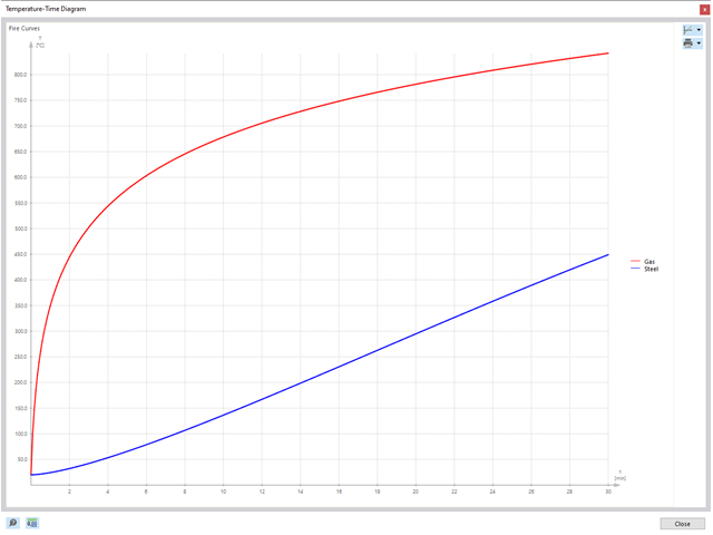
Na podstawie danych wejściowych można automatycznie określić decydującą temperaturę elementu w momencie przeprowadzania analizy. W takim przypadku można szczegółowo prześledzić krzywą temperatury w funkcji czasuwykres temperatura-czas.
.png?mw=640&hash=403c565ab80c4dd45c2d1356634fb74a90428b70)
W bibliotece konstrukcji warstwowych dostępni są następujący producenci drewna klejonego krzyżowo:
- Binderholz (USA)
- KLH (USA, CAN)
- Kalesnikoff (USA, CAN)
- Nordic Structures (USA, CAN)
- Mercer Mass Timber
- SmartLam
- Sterling Structural
- Konstrukcje nośne wymienione w Lignatec wydanie 32 "Drewno klejone krzyżowo z produkcji szwajcarskiej"
Wczytanie konstrukcji z biblioteki konstrukcji warstw powoduje automatyczne przejęcie wszystkich istotnych parametrów. Biblioteka jest stale aktualizowana.

W porównaniu z modułem dodatkowym RF-SOILIN (RFEM 5) do rozszerzenia Analiza geotechniczna dla programu RFEM 6 dodano następujące nowe funkcje:
- Tworzenie warstwowego gruntu jako modelu 3D z całości zdefiniowanych próbek gruntu
- Symulacja gruntu zgodnie z teorią Mohra-Coulomba
- Graficzne i tabelaryczne przedstawienie naprężeń i odkształceń na dowolnej głębokości gruntu
- Optymalne uwzględnienie interakcji gruntu i konstrukcji na podstawie modelu ogólnego
- 002171
- Ogólne informacje
- Projektowanie konstrukcji stalowych RFEM 6
- Projektowanie konstrukcji stalowych RSTAB 9
W porównaniu z modułem dodatkowym RF-/STEEL EC3 (RFEM 5/RSTAB 8) do rozszerzenia Wymiarowanie stali dla programu RFEM 6/RSTAB 9 dodano następujące nowe funkcje:
- Oprócz Eurokodu 3, uwzględnione zostały inne międzynarodowe normy (np. AISC 360, CSA S16, GB 50017, SP 16.13330)
- Berücksichtigung der Feuerverzinkung (DASt-Richtlinie 027) beim Brandschutznachweis nach EN 1993-1-2
- Opcja wprowadzania żeber usztywniających, które można uwzględnić w analizie wyboczenia
- Wyboczenie skrętne można również sprawdzić w przypadku przekrojów zamkniętych (np. istotne dla smukłych, wysokich prostokątnych przekrojów zamkniętych)
- Automatyczne wykrywanie prętów lub zbiorów prętów ważnych dla obliczeń (np. automatyczna dezaktywacja prętów z nieaktualnym materiałem lub prętów już zawartych w zbiorze prętów)
- Możliwość dostosowania ustawień obliczeniowych indywidualnie dla każdego pręta
- Graficzne przedstawienie wyników w przekroju brutto lub przekroju efektywnym
- Wyświetlanie odpowiednich wzorów użytych do sprawdzania warunków nośności (w tym odniesienie do zastosowanego równania z normy)
- 002333
- Ogólne informacje
- Projektowanie konstrukcji stalowych RFEM 6
- Projektowanie konstrukcji stalowych RSTAB 9
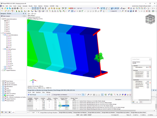
Rozszerzenie Skręcanie skrępowane (7 stopni swobody) oferuje szereg nowych opcji. W programach RFEM i RSTAB można na przykład przeprowadzić obliczenia konstrukcji prętowych z uwzględnieniem deplanacji przekroju. Wypadkowe siły wewnętrzne (N, Vu, Vv, Mt,pri, Mt,sec, Mu, Mv, Mω) można uwzględnić w analizie naprężeń równoważnych dla konstrukcji stalowych. Powiadomienia Funkcja ta nie jest obecnie dostępna dla norm projektowych AISC 360-16 i GB 50017.
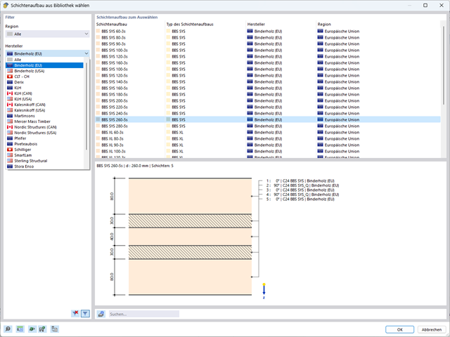
W programie RFEM zaimplementowano bibliotekę płyt z drewna klejonego krzyżowo, z której można importować konstrukcje warstwowe różnych producentów (np. Binderholz, KLH, Piveteaubois, Södra, Züblin Timber, Schilliger, Stora Enso). Oprócz grubości i materiałów warstw podane są również informacje o redukcji sztywności i łączeniu wąskich boków.
Przejdź do filmu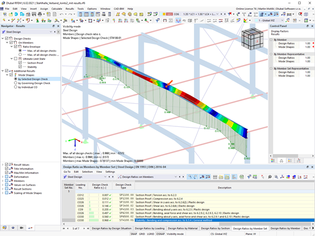
- 002335
- Ogólne informacje
- Projektowanie konstrukcji stalowych RFEM 6
- Projektowanie konstrukcji stalowych RSTAB 9
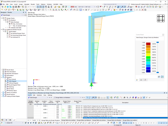
Czy do określenia współczynnika obciążenia krytycznego do analizy stateczności użyto solwera wartości własnych rozszerzenia? W ten sposób można wyświetlić decydujący kształt drgań własnych projektowanego obiektu. Na potrzeby analizy zwichrzenia dostępny jest solwer wartości własnych, w zależności od zastosowanej normy obliczeniowej. W przypadku metody ogólnej zgodnie z EN 1993-1-1, 6.3.4 można również użyć wewnętrznego solwera wartości własnych.
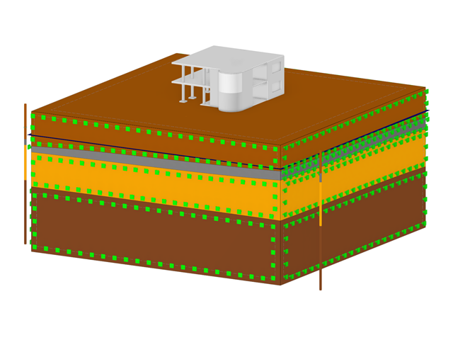
Bryły gruntu, które mają zostać przeanalizowane, są sumowane w masywach gruntu.
Próbki gruntu należy wykorzystać jako podstawę do zdefiniowania masywu gruntowego. W ten sposób program umożliwia generowanie masywu w sposób przyjazny dla użytkownika, w tym automatyczne określanie granic faz na podstawie danych z próbki, a także poziomu wód gruntowych i podpór powierzchni granicznej.
Masywy gruntowe umożliwiają określenie docelowego rozmiaru siatki ES niezależnie od ustawień globalnych dla reszty konstrukcji. Dzięki temu w całym modelu można uwzględnić różne wymagania dotyczące budynku i gruntu.
- 002131
- Obliczenia
- Projektowanie konstrukcji stalowych RFEM 6
- Projektowanie konstrukcji stalowych RSTAB 9
- Analiza stateczności dla wyboczenia giętnego, wyboczenia skrętnego i wyboczenia giętno-skrętnego przy ściskaniu
- Import długości efektywnych z obliczeń przy użyciu rozszerzenia Stateczność konstrukcji
- Graficzne wprowadzanie i kontrola zdefiniowanych podpór węzłowych oraz długości efektywnych w celu analizy stateczności
- Analiza zwichrzenia elementów poddanych obciążeniu momentem
- W zależności od normy istnieje wybór między wprowadzaniem wartości Mcr przez użytkownika, metodą analityczną z normy lub wykorzystaniem wewnętrznego solwera wartości własnych
- Uwzględnienie panelu usztywniającego i ograniczenia obrotu podczas korzystania z solwera wartości własnych
- Graficzne przedstawienie postaci własnej w przypadku zastosowania solwera wartości własnych
- Analiza stateczności elementów konstrukcyjnych ze ściskaniem i naprężeniem zginającym, w zależności od normy obliczeniowej
- Przejrzyste obliczenia wszystkich niezbędnych współczynników, takich jak współczynniki uwzględniające rozkładu momentów lub współczynniki interakcji
- Alternatywne uwzględnienie wszystkich wpływów dla analizy stateczności podczas określania sił wewnętrznych w programie RFEM/RSTAB (analiza drugiego rzędu, imperfekcje, redukcja sztywności, ewentualnie w połączeniu z rozszerzeniem Skręcanie skrępowane (7 stopni swobody))
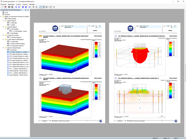
Twoje dane są zawsze dokumentowane w wielojęzycznym raporcie. W każdej chwili możesz dostosować treść i zapisać ją jako szablon. W raporcie można również za pomocą kilku kliknięć umieścić grafiki, teksty, wzory MathML i dokumenty PDF.
- 002319
- Ogólne informacje
- Projektowanie konstrukcji stalowych RFEM 6
- Projektowanie konstrukcji stalowych RSTAB 9
Zasady sprawdzania stanu granicznego użytkowalności można znaleźć w tabelach wyników w rozszerzeniu Projektowanie konstrukcji stalowych. Wyniki obliczeń można wyświetlić ze wszystkimi szczegółami w każdym miejscu obliczanych prętów. Ponadto dostępne są grafiki z wykresami wyników i stopni wykorzystania. Zapewnia to dobry przegląd sytuacji.
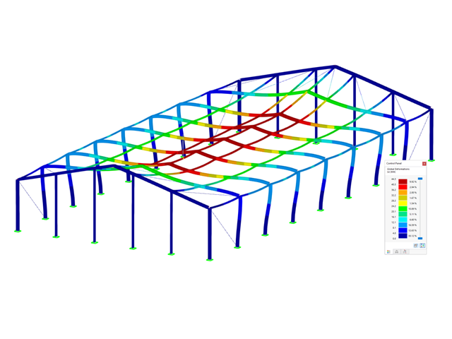
Wszystkie tabele wyników i grafiki można również zintegrować z globalnym protokołem wydruku programu RFEM/RSTAB jako część wyników wymiarowania stali. Dzięki temu można wyświetlać i dokumentować odkształcenia całej konstrukcji w ramach funkcji programu RFEM/RSTAB, niezależnie od rozszerzenia.
- 002334
- Ogólne informacje
- Projektowanie konstrukcji stalowych RFEM 6
- Projektowanie konstrukcji stalowych RSTAB 9
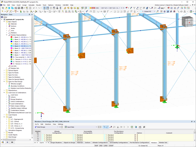
Czy chcesz przeprowadzić analizę stateczności w rozszerzeniu Projektowanie konstrukcji stalowych? W takim przypadku należy bezwzględnie zdefiniować długości efektywne. W tym celu w oknie wprowadzania danych należy zdefiniować podpory węzłowe i współczynniki długości efektywnej. W celu ułatwienia dokumentacji i kontroli wprowadzonych danych można również wyświetlić graficznie podpory węzłowe i powstałe w ten sposób segmenty wraz z odpowiednim współczynnikiem długości efektywnej w oknie roboczym programu RFEM/RSTAB.
- 002318
- Ogólne informacje
- Projektowanie konstrukcji stalowych RFEM 6
- Projektowanie konstrukcji stalowych RSTAB 9
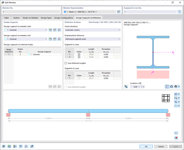
W programie RFEM/RSTAB istnieje możliwość wygenerowania, a następnie obliczenia kombinacji obciążeń lub wyników wymaganych dla stanu granicznego użytkowalności. Sytuacje obliczeniowe można wybrać do analizy ugięć w rozszerzeniu Projektowanie konstrukcji stalowych. Obliczone wartości odkształceń są odpowiednio określane w każdym miejscu pręta, w zależności od określonego wygięcia wstępnego i układu odniesienia. Na koniec można porównać te wartości odkształceń z wartościami granicznymi.
Czy wiecie, że...? Wartość graniczną deformacji można określić indywidualnie dla każdego elementu konstrukcyjnego w Konfiguracja stanu granicznego użytkowalności. Jako dopuszczalną wartość graniczną należy zdefiniować maksymalne odkształcenie w zależności od długości odniesienia. Poprzez zdefiniowanie podpór obliczeniowych można podzielić komponenty na segmenty w celu automatycznego określenia odpowiedniej długości odniesienia dla każdego kierunku obliczeń.
W zależności od położenia przydzielonych podpór obliczeniowych, rozróżnienie między belkami i wspornikami jest dokonywane automatycznie, dzięki czemu można odpowiednio określić wartość graniczną.
- 002332
- Ogólne informacje
- Projektowanie konstrukcji stalowych RFEM 6
- Projektowanie konstrukcji stalowych RSTAB 9
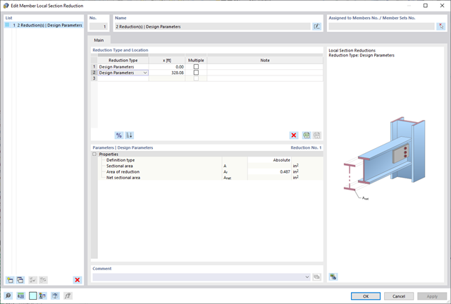
Należy pamiętać, że w przypadku łączenia elementów obciążonych rozciąganiem za pomocą połączeń śrubowych, w obliczeniach w stanie granicznym nośności należy uwzględnić redukcję przekroju ze względu na otwory na śruby. Ale bez obaw, można to łatwo zrobić w programie. W rozszerzeniu Projektowanie konstrukcji stalowych można wprowadzić lokalną redukcję przekroju pręta - i to wszystko. Redukcję przekroju można wprowadzić jako wartość bezwzględną lub jako procent całkowitej powierzchni we wszystkich istotnych miejscach.
- 002130
- Ogólne informacje
- Projektowanie konstrukcji stalowych RFEM 6
- Projektowanie konstrukcji stalowych RSTAB 9
- Wymiarowanie elementów rozciąganych, ściskanych, zginanych, ścinanych, skręcanych i poddanych połączonemu działaniu tych sił wewnętrznych
- Obliczanie rozciągania z uwzględnieniem zredukowanej powierzchni przekroju (np. osłabienie z uwagi na otwory)
- Automatyczna klasyfikacja przekrojów w celu sprawdzenia wyboczenia lokalnego
- Siły wewnętrzne z obliczeń ze skręcaniem skrępowanym (7 stopni swobody) są uwzględniane w kontroli naprężeń zastępczych (obecnie nie dla norm projektowych AISC 360-16 i GB 50017).
- Wymiarowanie przekrojów klasy 4 o właściwościach efektywnych zgodnie z EN 1993-1-5 oraz przekrojów formowanych na zimno zgodnie z EN 1993-1-3, AISI S100 lub CSA S136 (licencje dla RSECTION i "Przekroje efektywne" " są wymagane dla przekrojów RSECTION)
- Sprawdzenie wyboczenia przy ścinaniu zgodnie z EN 1993-1-5 z uwzględnieniem usztywnień poprzecznych
- Wymiarowanie elementów ze stali nierdzewnej zgodnie z EN 1993‑1-4
- 002331
- Ogólne informacje
- Projektowanie konstrukcji stalowych RFEM 6
- Projektowanie konstrukcji stalowych RSTAB 9
Rozszerzenie Projektowanie konstrukcji stalowych pomaga między innymi w wymiarowaniu ogólnych przekrojów, które nie są wstępnie zdefiniowane w bibliotece przekrojów. W tym celu należy utworzyć przekrój w programie RSECTION, a następnie zaimportować go do RFEM/RSTAB. W zależności od zastosowanej normy projektowej dostępne są różne formaty obliczeń. Jedną z nich jest na przykład analiza równoważnych naprężeń. Masz licencję na RSECTION i Przekroje efektywne? Następnie można przeprowadzić obliczenia z uwzględnieniem efektywnych właściwości przekrojów zgodnie z EN 1993-1-5.
W rozszerzeniu Projektowanie konstrukcji stalowych można przeprowadzić kontrolę obliczeń stateczności i przekrojów profili formowanych na zimno według EN 1993-1-3, zgodnie z punktami 6.1.2 - 6.1.5 i 6.1.8 - 6.1.10.
Przejdź do filmu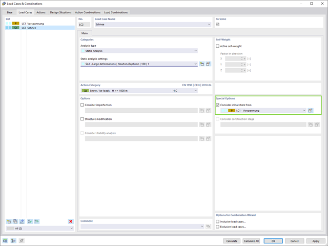
Czy wiesz dokładnie, w jaki sposób przebiega wyszukiwanie kształtu? Po pierwsze, proces znajdowania kształtu przypadków obciążeń z kategorią przypadku obciążenia "Wstępne naprężenie" przesuwa początkową geometrię siatki do optymalnie zrównoważonej pozycji za pomocą iteracyjnych pętli obliczeniowych. W tym celu program wykorzystuje metodę Zaktualizowanej Strategii Odniesienia (URS) opracowaną przez prof. Bletzingera i prof. Ramma. Technologię tę charakteryzują kształty równowagi, które po obliczeniach prawie dokładnie odpowiadają początkowo zadanym warunkom brzegowym (ugięcie, siła i naprężenie wstępne).
Oprócz opisu oczekiwanych sił lub zwisów na elementach, zintegrowane podejście URS umożliwia również uwzględnienie sił regularnych. W całym procesie pozwala to na przykład na opisanie ciężaru własnego lub ciśnienia pneumatycznego za pomocą odpowiednich obciążeń elementów.
Wszystkie te opcje dają rdzeniu obliczeniowemu możliwość obliczania postaci antyklastycznych i synklastycznych, które są w równowadze sił, dla geometrii płaskich lub obrotowo-symetrycznych. Aby możliwe było realistyczne zaimplementowanie obu typów, pojedynczo lub razem w jednym środowisku, w obliczeniach dostępne są dwa sposoby opisania wektorów sił do analizy form-finding:
- Metoda rozciągania - opis znajdowania kształtu wektorów sił w przestrzeni dla geometrii płaskich
- Metoda rzutowania - opis znajdowania kształtu wektorów sił na płaszczyznę rzutowania z ustaleniem położenia poziomego dla geometrii stożkowych
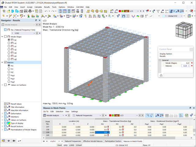
Czy odkryłeś już tabelaryczne i graficzne przedstawianie mas w punktach siatki? Po prawej, jest to również jeden z wyników analizy modalnej w programie RFEM 6. W ten sposób można sprawdzić importowane masy, które zależą od różnych ustawień analizy modalnej. Mogą być one wyświetlane w zakładce Masy w punktach siatki tabeli Wyniki. Tabela zawiera przegląd następujących wyników: Masa - kierunek przesuwny (mX, mY, mZ ), Masa - kierunek obrotowy (mφX, mφY, mφZ ) oraz suma mas. Czy nie byłoby lepiej, gdybyś jak najszybciej przeprowadził ocenę graficzną? Następnie można również wyświetlić graficznie masy w punktach siatki.
Wiesz już, że grunt i konstrukcję można modelować i analizować w całym modelu. Oznacza to, że wyraźnie uwzględniono interakcję gleba-konstrukcja. Dostosowanie jednego elementu konstrukcyjnego prowadzi do natychmiastowego prawidłowego uwzględnienia w analizie i wynikach dla całego układu gruntu i konstrukcji.