56 Wyniki
Wyświetl wyniki:
Sortuj według:
W rozszerzeniu Projektowanie konstrukcji betonowych można przeprowadzać obliczenia sejsmiczne dla prętów żelbetowych zgodnie z EC 8. Są to między innymi następujące funkcje:
- Konfiguracje obliczeń sejsmicznych
- Rozróżnianie klas ciągliwości DCL, DCM, DCH
- Możliwość przeniesienia współczynnika odpowiedzi z analizy dynamicznej
- Sprawdzenie wartości granicznej współczynnika odpowiedzi
- Weryfikacja nośności dla "Wytrzymały słup - słaba belka"
- Uszczegółowienie i reguły szczególne dla współczynnika ciągliwości krzywizny
- Uszczegółowienie i reguły szczególne dla ciągliwości lokalnej
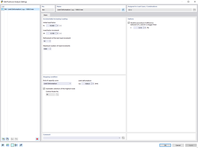
Analiza pushover jest zarządzana przez nowo wprowadzony typ analizy w kombinacjach obciążeń. W tym miejscu można wybrać poziomy rozkład i kierunek obciążenia, obciążenie stałe, żądane spektrum odpowiedzi do określenia docelowego przemieszczenia oraz ustawienia analizy pushover.
W ustawieniach analizy pushover można zmodyfikować przyrost obciążenia poziomego i określić warunek zatrzymania dla analizy. Ponadto użytkownik może bez problemu dostosować precyzyjność iteracyjnego definiowania przesunięcia docelowego.
- Uwzględnienie nieliniowego zachowania komponentu przy użyciu standardowych przegubów plastycznych dla stali (FEMA 356, EN 1998-3) i nieliniowego zachowania materiału (mur, stal - bilinearnie, krzywe robocze zdefiniowane przez użytkownika)
- Bezpośredni import mas z przypadków obciążeń lub kombinacji w celu przyłożenia stałych obciążeń pionowych
- Zdefiniowane przez użytkownika specyfikacje dotyczące uwzględniania obciążeń poziomych (ujednoliconych ze względu na postać drgań lub równomiernie rozłożonych na wysokości mas)
- Wyznaczanie krzywej pushover z możliwością wyboru kryterium granicznego obliczeń (zawalenie lub odkształcenie graniczne)
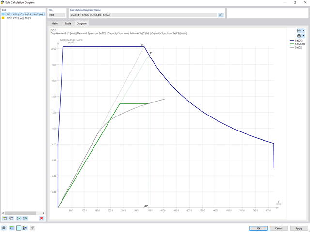
- Transformacja krzywej pushover w spektrum nośności (format ADRS, układ o jednym stopniu swobody)
- Bilinearyzacja spektrum nośności zgodnie z EN 1998-1:2010 + A1:2013
- Transformacja zastosowanego spektrum odpowiedzi w wymagane spektrum (format ADRS)
- Wyznaczanie docelowego przemieszczenia zgodnie z EC 8 (metoda N2 zgodnie z Fajfar 2000)
- Graficzne porównanie nośności i wymaganego spektrum
- Graficzna ocena kryteriów akceptacji zdefiniowanych przegubów plastycznych
- Wyświetlanie wyników obliczeń iteracyjnych docelowego przemieszczenia
- Dostęp do wszystkich wyników analizy statyczno-wytrzymałościowej w poszczególnych poziomach obciążenia
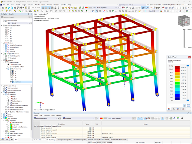
Podczas obliczeń wybrane obciążenie poziome jest zwiększane w krokach obciążenia. Statyczna analiza nieliniowa jest przeprowadzana dla każdego kroku obciążenia, aż do osiągnięcia określonego warunku granicznego.
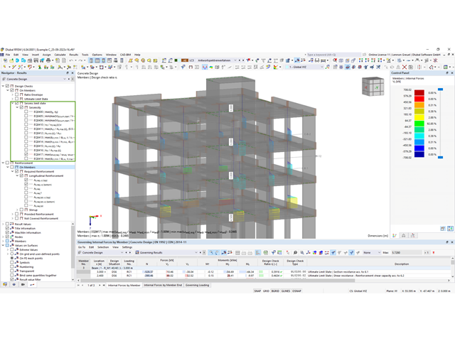
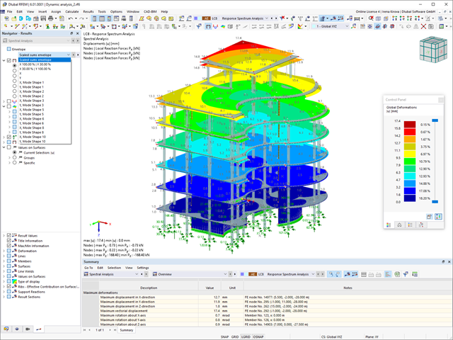
Wyniki analizy pushover są obszerne. Z jednej strony konstrukcja jest analizowana pod kątem odkstałceń. Można to przedstawić za pomocą linii siła-odkształcenie układu (krzywa nośności). Z drugiej strony, wpływ spektrum odpowiedzi można wyświetlić w oknie ADRS (Acceleration-Displacement Response Spectrum). Docelowe przemieszczenie jest określane w programie automatycznie na podstawie tych dwóch wyników. Proces można ocenić graficznie oraz w tabelach.
Poszczególne kryteria akceptacji można następnie przeanalizować i ocenić graficznie (dla następnego kroku obciążenia docelowego przemieszczenia, ale także dla wszystkich innych kroków obciążenia). Wyniki analizy statycznej są również dostępne dla poszczególnych kroków obciążenia.
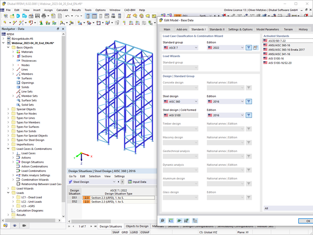
Wymiarowanie prętów stalowych formowanych na zimno zgodnie z AISI S100-16/CSA S136-16 jest dostępne w RFEM 6. Dostęp do obliczeń można uzyskać, wybierając normy „AISC 360” lub „CSA S16” w rozszerzeniu Projektowanie konstrukcji stalowych. Następnie dla obliczeń elementów formowanych na zimno automatycznie wybierane jest „AISI S100” lub „CSA S136”.
Do obliczania sprężystego obciążenia wyboczeniowego pręta program RFEM stosuje metodę DSM. Bezpośrednia metoda wytrzymałości oferuje dwa typy rozwiązań, numeryczne (metoda pasm skończonych) i analityczne (specyfikacja). Krzywą charakterystyczną (sygnaturę) FSM i kształty wyboczenia można wyświetlić w oknie dialogowym Przekroje.
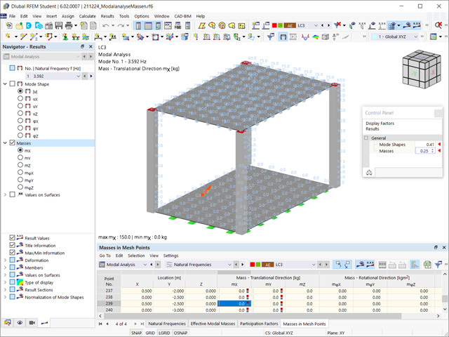
Czy odkryłeś już tabelaryczne i graficzne przedstawianie mas w punktach siatki? Po prawej, jest to również jeden z wyników analizy modalnej w programie RFEM 6. W ten sposób można sprawdzić importowane masy, które zależą od różnych ustawień analizy modalnej. Mogą być one wyświetlane w zakładce Masy w punktach siatki tabeli Wyniki. Tabela zawiera przegląd następujących wyników: Masa - kierunek przesuwny (mX, mY, mZ ), Masa - kierunek obrotowy (mφX, mφY, mφZ ) oraz suma mas. Czy nie byłoby lepiej, gdybyś jak najszybciej przeprowadził ocenę graficzną? Następnie można również wyświetlić graficznie masy w punktach siatki.
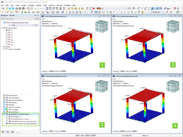
Jak już wiesz, po pomyślnym zakończeniu obliczeń wyniki przypadku obciążenia w Analizie modalnej są wyświetlane w programie. Die erste Eigenform ist für Sie also sofort grafisch oder animiert zu sehen. Dabei können Sie die Darstellung der Eigenformnormierung komfortabel anpassen. Erledigen Sie das am besten direkt im Ergebnisnavigator, wo Sie zur Visualisierung der Eigenformen eine von vier Optionen auswählen:
- Wert des Eigenformvektors uj auf 1 skalieren (berücksichtigt nur die Translationskomponenten)
- Auswahl der maximalen Translationskomponente des Eigenvektors und Einstellung auf 1
- Betrachtung der gesamten Eigenform (inklusive der Rotationskomponenten), Auswahl des Maximums und Einstellung auf 1
- Setzen der modalen Massen mi für jeden Eigenwert auf 1 kg
Ausführlichere Erläuterungen der Normierung der Eigenformen finden Sie hier: Instrukcja online .
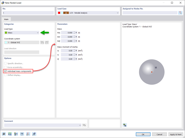
Czy oprócz obciążeń statycznych chcesz uwzględnić również inne obciążenia jako masy? Program umożliwia to dla obciążeń węzłowych, prętowych, liniowych i powierzchniowych. W tym celu podczas definiowania obciążenia należy wybrać typ Obciążenie masą. Dla takich obciążeń należy zdefiniować masę lub składowe masy w kierunkach X, Y i Z. W przypadku mas węzłowych można dodatkowo zdefiniować momenty bezwładności X, Y i Z w celu modelowania bardziej złożonych punktów mas.
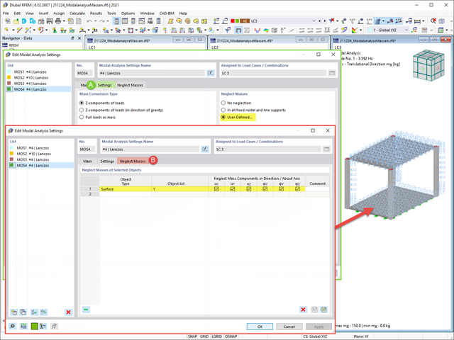
Często zachodzi potrzeba pominięcia mas. Dzieje się tak zwłaszcza w przypadku, gdy wyniki analizy modalnej mają być wykorzystane do analizy sejsmicznej. W tym celu wymagane jest 90% efektywnej masy modalnej w każdym kierunku. Pozwala to na pominięcie masy we wszystkich utwierdzonych podporach węzłowych i liniowych. Program automatycznie dezaktywuje powiązane masy.
Obiekty, których masy mają zostać pominięte w analizie modalnej, można również wybrać ręcznie. Dla lepszego widoku pokazaliśmy to ostatnie na rysunku. W wyniku wyboru przez użytkownika obiektów masowych wraz z skojarzonymi z nimi składowymi masowymi można pominąć masy.
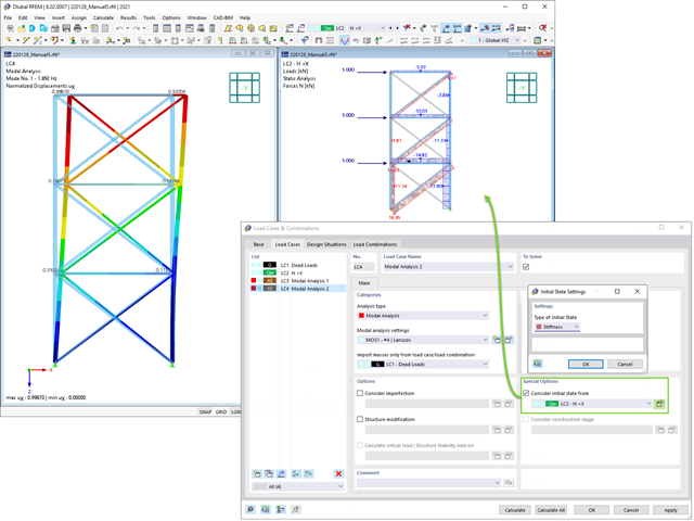
Podczas definiowania danych wejściowych dla przypadku obciążenia analizy modalnej można uwzględnić przypadek obciążenia, którego sztywności reprezentują początkową pozycję analizy modalnej. Jak to zrobić? Jak pokazano na rysunku, należy wybrać opcję "Uwzględnij stan początkowy z". Teraz otwórz okno dialogowe "Ustawienia stanu początkowego" i zdefiniuj typ Sztywność jako stan początkowy. W tym przypadku obciążenia, który jest stanem początkowym branym pod uwagę, można uwzględnić sztywność układu konstrukcyjnego, gdy pręty rozciągane ulegają uszkodzeniu. Celem tego wszystkiego: Sztywność z tego przypadku obciążenia jest uwzględniana w analizie modalnej. W ten sposób uzyskuje się wyraźnie elastyczny system.
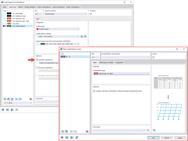
Widać to już na obrazku: Imperfekcje można również uwzględnić podczas definiowania przypadku obciążenia w analizie modalnej. Typy imperfekcji, które mogą być stosowane w analizie modalnej, to obciążenia hipotetyczne z przypadku obciążenia, początkowe przemieszczenie w tabeli, odkształcenie statyczne, postać wyboczeniowa, postać dynamiczna oraz grupa przypadków imperfekcji.
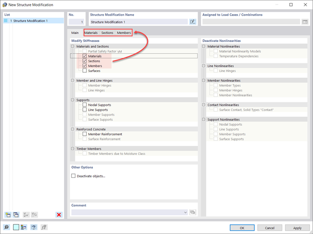
Czy wiecie, że...? W przypadkach obciążeń typu Analiza modalna można z łatwością wprowadzać zmiany konstrukcyjne. Pozwala to na przykład na indywidualne dostosowanie sztywności materiałów, przekrojów, prętów, powierzchni, przegubów i podpór. W przypadku niektórych rozszerzeń można również modyfikować sztywności. Po wybraniu obiektów ich właściwości sztywności są dostosowywane do typu obiektu. W ten sposób można je zdefiniować w osobnych zakładkach.
Czy chcesz przeanalizować uszkodzenie obiektu (na przykład słupa) w analizie modalnej? Jest to również możliwe bez żadnych problemów. Wystarczy przejść do okna Modyfikacja konstrukcji i dezaktywować odpowiednie obiekty.
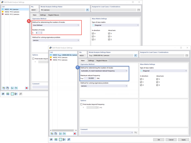
Twoim celem jest określenie liczby postaci drgań własnych? Program oferuje dwie metody. Z jednej strony, można ręcznie zdefiniować liczbę najmniejszych kształtów drgań, które mają zostać obliczone. W tym przypadku liczba dostępnych kształtów postaci zależy od stopni swobody (tzn. liczby punktów mas swobodnych pomnożonych przez liczbę kierunków, w których działają masy). Jest to jednak ograniczone do 9999. Z drugiej strony, maksymalną częstotliwość drgań własnych można ustawić w taki sposób, w jaki program określił kształty automatycznie, aż do osiągnięcia zadanej częstotliwości drgań własnych.
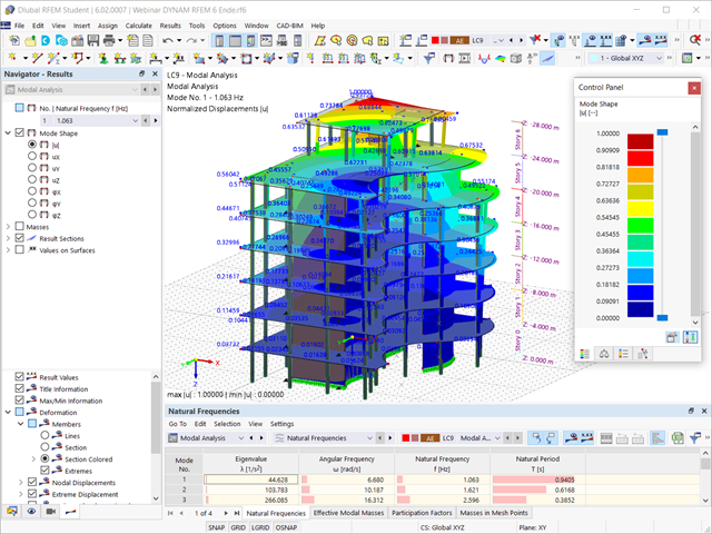
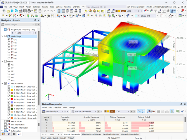
Czy obliczenia się zakończyły? Wyniki analizy modalnej są wówczas dostępne zarówno w formie graficznej, jak i tabelarycznej. Wyświetl tabele wyników dla przypadku obciążenia lub przypadków obciążeń analizy modalnej. Dzięki temu na pierwszy rzut oka można zobaczyć wartości własne, częstotliwości kątowe, częstotliwości i okresy drgań własnych konstrukcji. W przejrzysty sposób wyświetlane są również efektywne masy modalne, modalne współczynniki masy i współczynniki udziału.
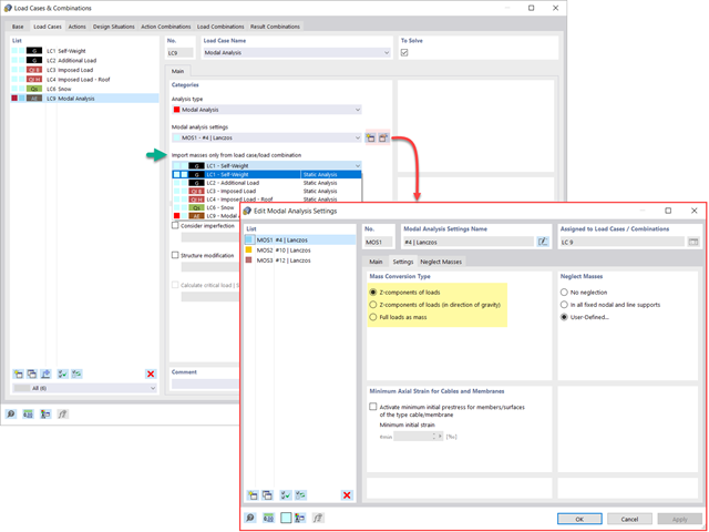
Dostępnych jest kilka opcji definiowania mas dla analizy modalnej. Masy od ciężaru własnego są uwzględniane automatycznie, natomiast obciążenia i masy można uwzględnić bezpośrednio w przypadku obciążenia typu analiza modalna. Potrzebujesz więcej opcji? Należy wybrać, czy obciążenia pełne mają być uwzględniane jako masy, składowe obciążenia w globalnym kierunku Z, czy tylko składowe obciążenia w kierunku siły ciężkości.
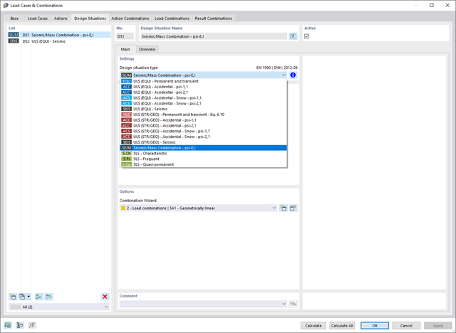
Program oferuje dodatkową lub alternatywną opcję importu mas: Ręczna definicja kombinacji obciążeń, począwszy od których masy są uwzględniane w analizie modalnej. Wybrałeś normę obliczeniową? Następnie można utworzyć sytuację obliczeniową typu Kombinacja mas sejsmicznych. W ten sposób program automatycznie oblicza sytuację masową dla analizy modalnej zgodnie z preferowaną normą obliczeniową. Innymi słowy: Program tworzy kombinację obciążeń na podstawie współczynników kombinacji wstępnie ustawionych dla wybranej normy. Zawiera on masy użyte do analizy modalnej.
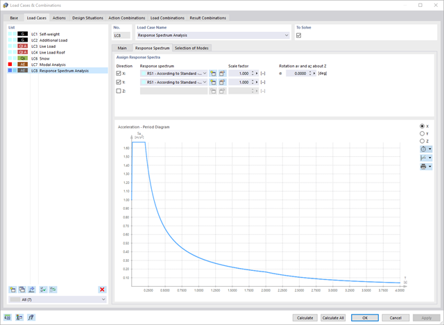
Oprogramowanie do analizy statyczno-wytrzymałościowej firmy Dlubal wykonuje wiele pracy za Ciebie. Program sugeruje zgodnie z regułami parametry wejściowe, istotne dla wybranych norm. Ponadto można ręcznie wprowadzić spektra odpowiedzi.
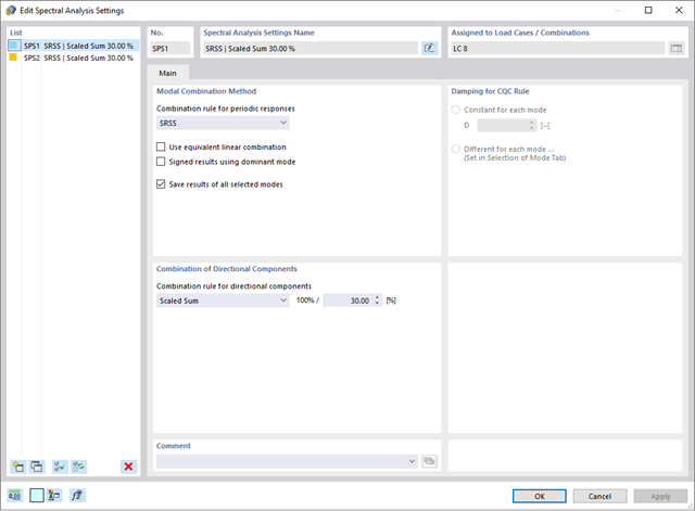
Przypadki obciążeń typu Analiza spektrum odpowiedzi określają kierunek, w którym działają spektra odpowiedzi oraz które wartości własne konstrukcji są istotne dla analizy. W ustawieniach analizy spektralnej można zdefiniować szczegóły dotyczące reguł kombinacji, tłumienia (jeśli ma zastosowanie) i przyspieszenia okresu zerowego (ZPA).
Czy wiecie, że...? Równoważne obciążenia statyczne generowane są oddzielnie dla każdej miarodajnej postaci drgań własnych oraz kierunku wzbudzenia. Obciążenia te są zapisywane w przypadku obciążenia typu Analiza spektrum odpowiedzi, a program RFEM/RSTAB przeprowadza liniową analizę statyczną.
Przypadki obciążeń typu Analiza spektrum odpowiedzi zawierają wygenerowane obciążenia równoważne. Po pierwsze, udziały modalne muszą zostać nałożone na siebie z regułą SRSS lub CQC. W takim przypadku można wykorzystać wyniki podpisane na podstawie dominującego kształtu drgań.
Następnie składowe kierunkowe oddziaływań sejsmicznych są łączone z regułą SRSS lub regułą 100%/30%.
- Automatyczne uwzględnianie masy własnej od ciężaru konstrukcji
- Możliwy bezpośredni import mas z przypadków obciążeń lub kombinacji
- Opcjonalne definiowanie mas dodatkowych (masy węzłowe, liniowe lub powierzchniowe oraz masy wynikające z bezwładności) bezpośrednio w przypadkach obciążeń
- Opcjonalne pominięcie mas (na przykład masy fundamentów)
- Kombinacje mas w różnych przypadkach i kombinacjach obciążeń
- Predefiniowane współczynniki kombinacji wg różnych norm (EC 8, SIA 261, ASCE 7, ...)
- Opcjonalny import stanów początkowych (np. w celu uwzględnienia naprężenia wstępnego i imperfekcji)
- modyfikacja konstrukcji
- Uwzględnianie uszkodzenia w podporach lub prętach/powierzchniach/bryłach
- Możliwość zadania kilku analiz modalnych (np. w celu analizy różnych mas lub modyfikacji sztywności)
- Wybór typu macierzy mas (macierz diagonalna, macierz spójna, macierz jednostkowa) oraz wskazanych przez użytkownika stopni swobody (translacyjne i rotacyjne)
- Metody określania liczby postaci drgań własnych (liczba zdefiniowana przez użytkownika, liczba określana automatycznie - w celu osiągnięcia zadanych efektywnych współczynników masy modalnej, liczba określana automatycznie - w celu osiągnięcia maksymalnej częstotliwości drgań własnych - dostępne tylko w programie RSTAB)
- Określanie postaci drgań i mas w węzłach siatki MES
- Wyniki w postaci wartości własnych, częstości kątowych, częstotliwości drgań własnych i okresu drgań własnych
- Wyniki w postaci mas modalnych, efektywnych mas modalnych, współczynników masy modalnej i współczynników udziału masy
- Tabelaryczne i graficzne przedstawienie mas w punktach siatki MES
- Wizualizacja i animacja postaci drgań własnych
- Różne opcje skalowania postaci drgań własnych
- Dokumentacja wyników numerycznych i graficznych w raporcie
W ustawieniach analizy modalnej należy wprowadzić wszystkie dane, które są niezbędne do określenia częstotliwości drgań własnych. Są to na przykład kształty mas i solwery wartości własnych.
Rozszerzenie Analiza modalna określa najniższe wartości częstości drgań własnych konstrukcji. Liczbę wartości własnych można dostosować lub określić automatycznie. Należy zatem osiągnąć efektywne współczynniki masy modalnej lub maksymalne częstotliwości drgań własnych. Masy są importowane bezpośrednio z przypadków obciążeń i kombinacji obciążeń. W takim przypadku istnieje możliwość uwzględnienia masy całkowitej, składowych obciążenia w globalnym kierunku Z lub tylko składowej obciążenia w kierunku siły ciężkości.
Dodatkowe masy w węzłach, liniach, prętach lub powierzchniach można zdefiniować ręcznie. Ponadto można wpływać na macierz sztywności poprzez import sił osiowych lub modyfikacji sztywności z przypadku obciążenia lub kombinacji obciążeń.
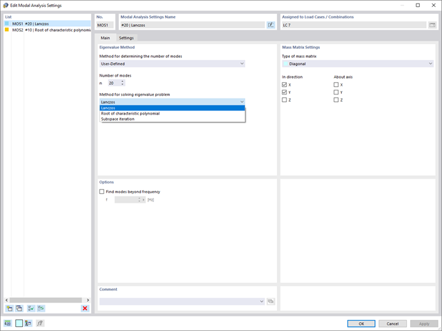
W programie RFEM dostępne są trzy wydajne solwery wartości własnych:
- pierwiastek wielomianu charakterystycznego
- Metoda Lanchosa
- iteracja podprzestrzeni
Z kolei program RSTAB oferuje dwa solwery wartości własnych:
- iteracja podprzestrzeni
- Metoda Powera z przesuniętą odwrotnością
Wybór solwera wartości własnych zależy przede wszystkim od rozmiaru modelu.
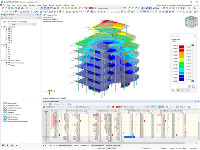
Zaraz po zakończeniu obliczeń wyświetlane są wartości własne, częstotliwości drgań własnych i okresy. Okna z tymi wynikami zintegrowane są z programem głównym RFEM/RSTAB. W tabelach można znaleźć wszystkie kształty drgań konstrukcji, a także można je wyświetlić graficznie i animować.
Wszystkie tabele wyników i grafiki stanowią część raportu programu RFEM/RSTAB. Zapewnia to przejrzystą dokumentację obliczeń. Tabele można również eksportować do programu MS Excel.
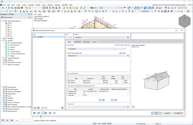
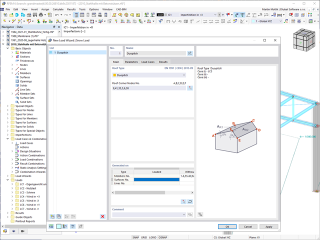
Czy chcesz, aby Twoje konstrukcje pozostały pionowe nawet podczas wiatru i śniegu? W takim razie skorzystaj z generatorów obciążeń dla konstrukcji płytowych i ramowych. Teraz można generować obciążenia wiatrem zgodnie z EN 1991‑1-4 oraz obciążenia śniegiem zgodnie z EN 1991‑1‑3 (a także innymi normami międzynarodowymi). Przypadki obciążeń są generowane w zależności od kształtu dachu.
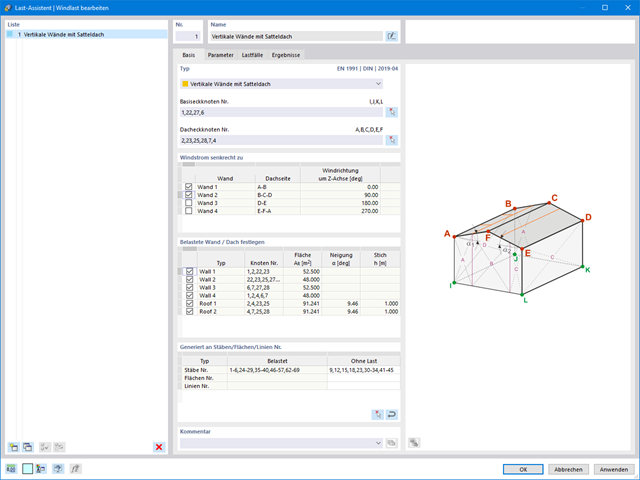
Obciążenia wiatrem również nie stanowią problemu w obliczeniach. Obciążenia wiatrem mogą być generowane automatycznie jako obciążenia prętowe lub obciążenia powierzchniowe (RFEM) na następujących elementach konstrukcyjnych:
- Ściany pionowe
- Dachy płaskie
- Dachy jednospadowe
- Dachy dwuspadowe/korytowe
- Ściany pionowe z dachem dwuspadowym
- Ściany pionowe z dachem płaskim/jednospadowym
Dostępne są następujące normy:
-
 EN 1991-1-4 (wraz z załącznikami krajowymi)
 -
 ASCE 7
 -
 NBC
NBC -
 CTE DB-SE-AE
 -
 GB 50009
Czy Twoje konstrukcje również muszą wytrzymać opady śniegu? Za pomocą Kreatora obciążeń śniegiem można generować obciążenia śniegiem jako obciążenia prętowe lub powierzchniowe.
Dostępne są poniższe normy:
-
EN 1991-1-3 (wraz z załącznikami krajowymi)
-
ASCE 7
-
NBC
-
 SIA 261
 -
CTE DB-SE-AE
-
GB 50009
-
 IS 875
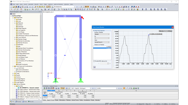
Dzięki integracji RF-/DYNAM Pro z programem RFEM lub RSTAB, do globalnego raportu można włączać numeryczne i graficzne wyniki z RF-/DYNAM Pro - Nonlinear Time History. Ponadto wszystkie opcje w programach RFEM i RSTAB są dostępne do wizualizacji graficznej. Wyniki analizy przebiegu czasowego wyświetlane są na wykresie przebiegu czasowego.
Wyniki są wyświetlane w funkcji czasu, a wartości liczbowe można eksportować do programu MS Excel. Kombinacje wyników mogą być eksportowane jako wynik pojedynczego kroku czasowego lub najbardziej niekorzystne wyniki wszystkich kroków czasowych są odfiltrowywane.
Obliczenia w RFEM
Nieliniowa analiza przebiegu czasowego jest przeprowadzana za pomocą pośredniej analizy Newmarka lub analizy bezpośredniej. Obie metody są metodami bezpośredniej integracji czasu. Analiza pośrednia wymaga definiowania małych kroków czasowych w celu dostarczenia dokładnych wyników. Analiza bezpośrednia określa automatycznie wymagany krok czasowy, w celu zapewnienia stabilności rozwiązania. Analizę bezpośrednią stosuje się w przypadku obliczania krótkotrwałych wzbudzeń, takich jak wzbudzenia impulsowe lub wybuch.
Obliczenia w RSTAB
Nieliniowa analiza przebiegu czasowego jest przeprowadzana z wykorzystaniem analizy bezpośredniej. Jest to metoda bezpośredniej integracji czasu i określa automatycznie krok czasowy, konieczny w celu zapewnienia stabilności wyników obliczeń.

- 001351
- Moduły dodatkowe
- RF-Dynam Pro (en) | Nieliniowa historia czasowa 5
- Analiza dynamiczna i sejsmiczna
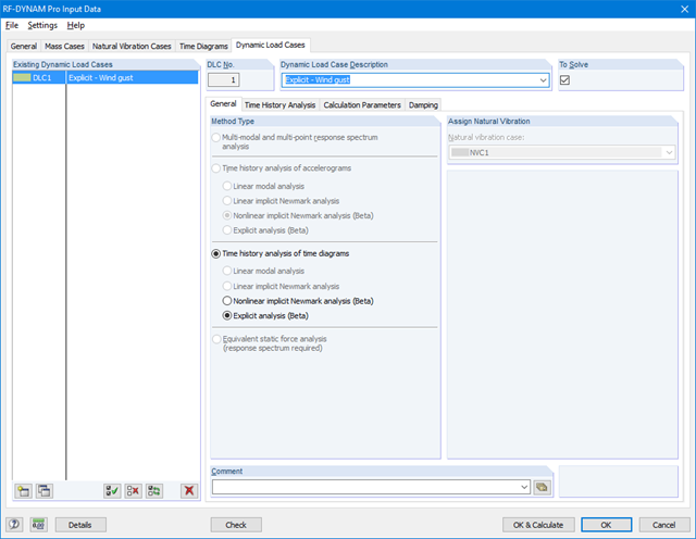
RF-/DYNAM Pro - Nonlinear Time History jest zintegrowany z RF‑/DYNAM Pro - Forced Vibrations i rozszerzony o dwie metody analizy nieliniowej (jedna analiza nieliniowa w RSTAB).
Wykresy siła-czas mogą być wprowadzane jako przejściowe, okresowe lub jako funkcje czasu. Dynamiczne przypadki obciążeń stanowią połączenie wykresów czasowych ze statycznymi przypadkami obciążeń, co zapewnia dużą elastyczność. Ponadto, istnieje możliwość definiowania kroków czasowych do obliczeń, tłumienia konstrukcji i opcji eksportu w dynamicznych przypadkach obciążeń.

- 001349
- Ogólne informacje
- RF-Dynam Pro (en) | Nieliniowa historia czasowa 5
- Analiza dynamiczna i sejsmiczna
- Nieliniowe typy prętów, takie jak pręty ściskane i rozciągane lub kable
- Nieliniowości pręta, takie jak uszkodzenie, przerwanie, uplastycznienie pod wpływem rozciągania lub ściskania
- Nieliniowości podpory, takie jak uszkodzenie, tarcie, wykres i częściowa aktywność
- Nieliniowości zwolnienia, takie jak tarcie, częściowa aktywność, wykres oraz uszkodzenie w przypadku, gdy siły wewnętrzne są dodatnie lub ujemne
.png?mw=640&hash=8cfd0c4bd093c03de543d147ffbf6f5c9250634a)
- 001348
- Ogólne informacje
- RF-Dynam Pro (en) | Nieliniowa historia czasowa 5
- Analiza dynamiczna i sejsmiczna
- Zdefiniowane przez użytkownika wykresy czasowe w funkcji czasu, w formie tabelarycznej lub jako obciążenia harmoniczne
- Połączenie wykresów czasowych z przypadkami lub kombinacjami obciążeń w programie RFEM/RSTAB (definiowanie obciążeń węzłowych, prętowych i powierzchniowych oraz zmiennych w czasie obciążeń wolnych i obciążeń)
- Możliwość połączenia kilku niezależnych oddziaływań wzbudzonych
- Nieliniowa analiza przebiegu czasowego z niejawną analizą Newmarka (tylko w RFEM) lub analizą bezpośrednią
- Tłumienie konstrukcji przy użyciu współczynnika Rayleigha lub tłumienia Lehra's
- Bezpośredni import początkowych deformacji z przypadku obciążenia lub kombinacji obciążeń (tylko RFEM)
- Modyfikacje sztywności jako warunki początkowe; na przykład wpływ siły osiowej, dezaktywowane pręty (tylko RSTAB)
- Graficzne przedstawienie rezultatów na diagramie przebiegu czasowego
- Eksport wyników w zdefiniownych przez użytkownika krokach czasowych lub jako obwiednia