85 Wyniki
Wyświetl wyniki:
Sortuj według:
W rozszerzeniu Projektowanie konstrukcji betonowych można przeprowadzać obliczenia sejsmiczne dla prętów żelbetowych zgodnie z EC 8. Są to między innymi następujące funkcje:
- Konfiguracje obliczeń sejsmicznych
- Rozróżnianie klas ciągliwości DCL, DCM, DCH
- Możliwość przeniesienia współczynnika odpowiedzi z analizy dynamicznej
- Sprawdzenie wartości granicznej współczynnika odpowiedzi
- Weryfikacja nośności dla "Wytrzymały słup - słaba belka"
- Uszczegółowienie i reguły szczególne dla współczynnika ciągliwości krzywizny
- Uszczegółowienie i reguły szczególne dla ciągliwości lokalnej
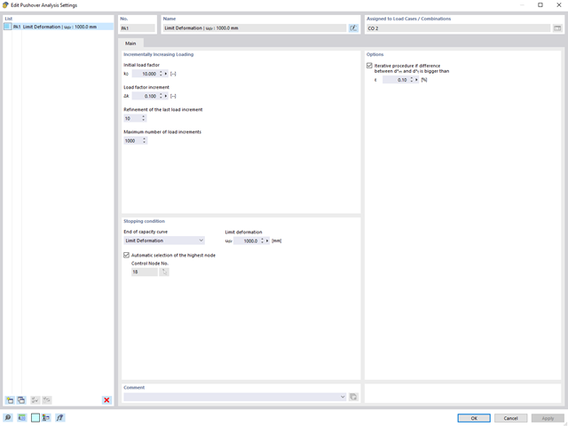
Analiza pushover jest zarządzana przez nowo wprowadzony typ analizy w kombinacjach obciążeń. W tym miejscu można wybrać poziomy rozkład i kierunek obciążenia, obciążenie stałe, żądane spektrum odpowiedzi do określenia docelowego przemieszczenia oraz ustawienia analizy pushover.
W ustawieniach analizy pushover można zmodyfikować przyrost obciążenia poziomego i określić warunek zatrzymania dla analizy. Ponadto użytkownik może bez problemu dostosować precyzyjność iteracyjnego definiowania przesunięcia docelowego.
- Uwzględnienie nieliniowego zachowania komponentu przy użyciu standardowych przegubów plastycznych dla stali (FEMA 356, EN 1998-3) i nieliniowego zachowania materiału (mur, stal - bilinearnie, krzywe robocze zdefiniowane przez użytkownika)
- Bezpośredni import mas z przypadków obciążeń lub kombinacji w celu przyłożenia stałych obciążeń pionowych
- Zdefiniowane przez użytkownika specyfikacje dotyczące uwzględniania obciążeń poziomych (ujednoliconych ze względu na postać drgań lub równomiernie rozłożonych na wysokości mas)
- Wyznaczanie krzywej pushover z możliwością wyboru kryterium granicznego obliczeń (zawalenie lub odkształcenie graniczne)
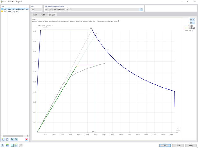
- Transformacja krzywej pushover w spektrum nośności (format ADRS, układ o jednym stopniu swobody)
- Bilinearyzacja spektrum nośności zgodnie z EN 1998-1:2010 + A1:2013
- Transformacja zastosowanego spektrum odpowiedzi w wymagane spektrum (format ADRS)
- Wyznaczanie docelowego przemieszczenia zgodnie z EC 8 (metoda N2 zgodnie z Fajfar 2000)
- Graficzne porównanie nośności i wymaganego spektrum
- Graficzna ocena kryteriów akceptacji zdefiniowanych przegubów plastycznych
- Wyświetlanie wyników obliczeń iteracyjnych docelowego przemieszczenia
- Dostęp do wszystkich wyników analizy statyczno-wytrzymałościowej w poszczególnych poziomach obciążenia
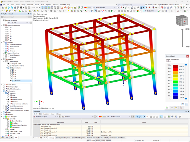
Podczas obliczeń wybrane obciążenie poziome jest zwiększane w krokach obciążenia. Statyczna analiza nieliniowa jest przeprowadzana dla każdego kroku obciążenia, aż do osiągnięcia określonego warunku granicznego.
Wyniki analizy pushover są obszerne. Z jednej strony konstrukcja jest analizowana pod kątem odkstałceń. Można to przedstawić za pomocą linii siła-odkształcenie układu (krzywa nośności). Z drugiej strony, wpływ spektrum odpowiedzi można wyświetlić w oknie ADRS (Acceleration-Displacement Response Spectrum). Docelowe przemieszczenie jest określane w programie automatycznie na podstawie tych dwóch wyników. Proces można ocenić graficznie oraz w tabelach.
Poszczególne kryteria akceptacji można następnie przeanalizować i ocenić graficznie (dla następnego kroku obciążenia docelowego przemieszczenia, ale także dla wszystkich innych kroków obciążenia). Wyniki analizy statycznej są również dostępne dla poszczególnych kroków obciążenia.
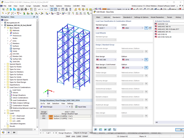
Wymiarowanie prętów stalowych formowanych na zimno zgodnie z AISI S100-16/CSA S136-16 jest dostępne w RFEM 6. Dostęp do obliczeń można uzyskać, wybierając normy „AISC 360” lub „CSA S16” w rozszerzeniu Projektowanie konstrukcji stalowych. Następnie dla obliczeń elementów formowanych na zimno automatycznie wybierane jest „AISI S100” lub „CSA S136”.
Do obliczania sprężystego obciążenia wyboczeniowego pręta program RFEM stosuje metodę DSM. Bezpośrednia metoda wytrzymałości oferuje dwa typy rozwiązań, numeryczne (metoda pasm skończonych) i analityczne (specyfikacja). Krzywą charakterystyczną (sygnaturę) FSM i kształty wyboczenia można wyświetlić w oknie dialogowym Przekroje.
- 002469
- Ogólne informacje
- Projektowanie konstrukcji betonowych RFEM 6
- Projektowanie konstrukcji betonowych RSTAB 9
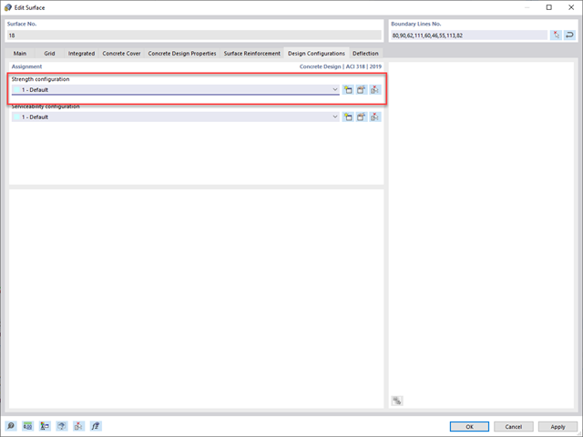
Pracujesz z elementami konstrukcyjnymi składającymi się z płyt? W takim przypadku należy przeprowadzić obliczenia na ścinanie z uwzględnieniem wymagań obliczania przebicia, na przykład zgodnie z 6.4, EN 1992-1-1. Oprócz płyt stropowych można w ten sposób wymiarować również płyty fundamentowe.
W konfiguracji stanu granicznego nośności dla wymiarowania betonu można zdefiniować parametry obliczeń przebicia dla wybranych węzłów.
- 002457
- Ogólne informacje
- Projektowanie konstrukcji aluminiowych RFEM 6
- Projektowanie konstrukcji aluminiowych RSTAB 9
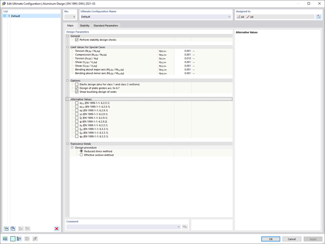
Rozszerzenie Projektowanie konstrukcji aluminiowych oferuje dodatkowe opcje. W tym miejscu można również obliczać przekroje ogólne, które nie są wstępnie zdefiniowane w bibliotece przekrojów. Na przykład, utwórz przekrój w programie RSECTION, a następnie zaimportuj go do RFEM/RSTAB. W zależności od zastosowanej normy projektowej dostępne są różne formaty obliczeń. Obejmuje to na przykład równoważną analizę naprężeń.
Ist zudem eine Lizenz für RSECTION und „Effektive Querschnitte“ vorhanden, so können Sie die Nachweise auch unter Berücksichtigung der effektiven Querschnittswerte nach EN 1999-1-1 führen.
- 002458
- Ogólne informacje
- Projektowanie konstrukcji aluminiowych RFEM 6
- Projektowanie konstrukcji aluminiowych RSTAB 9
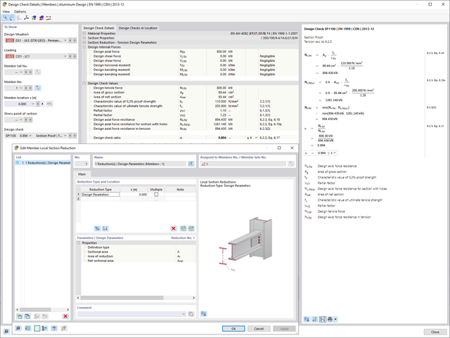
Wiesz na pewno, że podczas łączenia elementów rozciąganych za pomocą połączeń śrubowych należy wziąć pod uwagę osłabienie przekroju spowodowane otworami na śruby. Programy do analizy statyczno-wytrzymałościowej również mają na to rozwiązanie. W rozszerzeniu Aluminium Design można wprowadzić lokalną redukcję przekroju pręta. Redukcję przekroju należy wprowadzić jako wartość bezwzględną lub jako procent powierzchni całkowitej.
- 002459
- Ogólne informacje
- Projektowanie konstrukcji aluminiowych RFEM 6
- Projektowanie konstrukcji aluminiowych RSTAB 9
Rozszerzenie Skręcanie skrępowane (7 stopni swobody) umożliwia przeprowadzanie obliczeń konstrukcji prętowych w programach RFEM i RSTAB, z uwzględnieniem deplanacji przekrojów. Wszystkie siły wewnętrzne (N, Vu, Vv, Mt, pri, Mt, sec, Mu, Mv, Mω) określone w ten sposób mogą zostać uwzględnione w analizie naprężeń zastępczych dla obliczeń konstrukcji aluminiowych. Uwaga: Ta funkcja nie jest jeszcze dostępna dla norm projektowych ADM 2020.
- 002462
- Ogólne informacje
- Projektowanie konstrukcji aluminiowych RFEM 6
- Projektowanie konstrukcji aluminiowych RSTAB 9
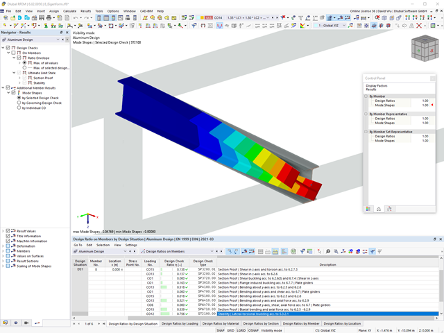
Czy do określenia współczynnika obciążenia krytycznego w ramach analizy stateczności użyto dodatkowego solwera wewnętrznych wartości własnych? W takim przypadku można następnie wyświetlić kształt wzorca projektowanego obiektu.
- 002451
- Ogólne informacje
- Projektowanie konstrukcji aluminiowych RFEM 6
- Projektowanie konstrukcji aluminiowych RSTAB 9
- Obliczanie ugięć i porównanie z normatywnymi lub ręcznie dostosowanymi wartościami granicznymi
- Uwzględnienie wygięcia wstępnego w analizie ugięcia
- W zależności od typu sytuacji obliczeniowej możliwe są różne wartości graniczne
- Ręczne dostosowywanie długości odniesienia i segmentacji według kierunku
- Obliczenia ugięć w odniesieniu do konstrukcji wyjściowej lub konstrukcji odkształconej
- Dalsze szczegółowe weryfikacje w zależności od wybranej normy obliczeniowej (np. weryfikacja drgań zgodnie z EN 1999-1-1, 7.2.3)
- Graficzne wyświetlanie wyników zintegrowane w programie RFEM/RSTAB, na przykład stopień wykorzystania wartości granicznej, odkształcenie lub ugięcie
- Pełna integracja wyników z raportem RFEM/RSTAB
- 002452
- Ogólne informacje
- Projektowanie konstrukcji aluminiowych RFEM 6
- Projektowanie konstrukcji aluminiowych RSTAB 9
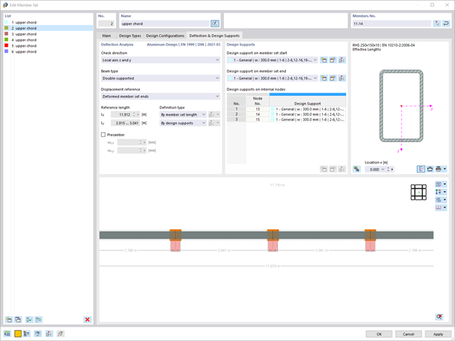
Program wykonuje za Ciebie dużo pracy. Na przykład kombinacje obciążeń lub wyników, które są niezbędne dla stanu granicznego użytkowalności, są generowane i obliczane w programie RFEM/RSTAB. Te sytuacje obliczeniowe można wybrać w rozszerzeniu Aluminium Design w celu przeprowadzenia analizy ugięcia. W zależności od wprowadzonej przechyłki i wybranego układu odniesienia program określa obliczone wartości deformacji w każdym punkcie pręta. Następnie są one porównywane z wartościami granicznymi.
W konfiguracji Stan graniczny użytkowalności można ustawić wartość graniczną, która ma być obserwowana dla odkształcenia dla każdego komponentu z osobna. Jako dopuszczalną wartość graniczną definiuje się maksymalne odkształcenie w zależności od długości odniesienia. Definiując podpory obliczeniowe, można segmentować komponenty. W ten sposób można automatycznie określić odpowiednią długość odniesienia dla każdego kierunku obliczeń.
To nie wszystko. W oparciu o położenie przypisanych podpór obliczeniowych program automatycznie umożliwia rozróżnienie belek i belek wspornikowych. W ten sposób określana jest odpowiednio wartość graniczna.
- 002453
- Ogólne informacje
- Projektowanie konstrukcji aluminiowych RFEM 6
- Projektowanie konstrukcji aluminiowych RSTAB 9
Obliczenia w stanie granicznym użytkowalności można znaleźć w tabelach wyników w rozszerzeniu do obliczeń dla aluminium. Są tam już w pełni zintegrowane. Istnieje możliwość uzyskania wyników obliczeń w każdym punkcie wymiarowanych prętów ze wszystkimi szczegółami. Można również użyć grafiki z wynikami współczynników obliczeniowych.
W razie potrzeby wszystkie tabele wyników i grafiki można uwzględnić jako część wyników obliczeń aluminium w globalnym raporcie wydruku programu RFEM/RSTAB. Program RFEM/RSTAB umożliwia również wyświetlanie i dokumentowanie wartości deformacji całej konstrukcji niezależnie od tego, czy jest to moduł dodatkowy.
- 002454
- Ogólne informacje
- Projektowanie konstrukcji aluminiowych RFEM 6
- Projektowanie konstrukcji aluminiowych RSTAB 9
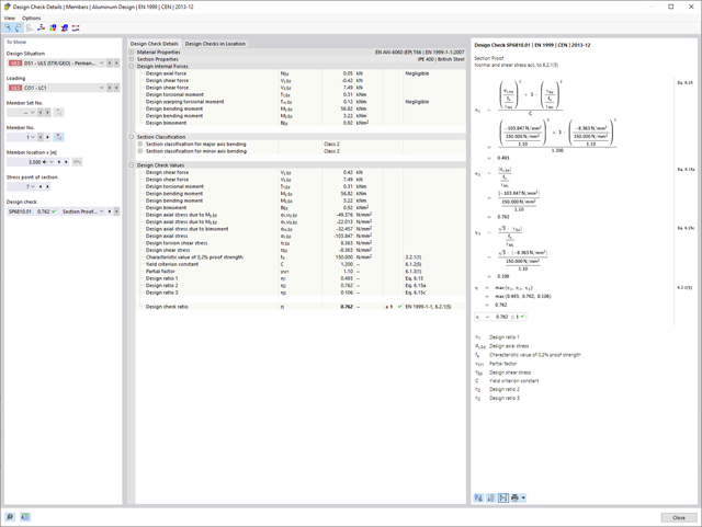
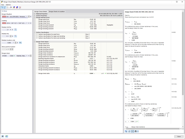
Czy bardzo to lubisz? My też! Z tego powodu wszystkie sprawdzenia dotyczące normy projektowej są wyświetlane w przejrzysty sposób. Dla każdej kontroli obliczeń należy zdefiniować kryterium wykorzystania. Szczegóły obliczeń, w których wartości wejściowe, wyniki pośrednie i wyniki końcowe są uporządkowane w sposób uporządkowany, są dostępne dla każdej kontroli obliczeń. Proces obliczeń wraz ze wszystkimi wzorami, normami i wynikami znajduje się w oknie informacyjnym, w którym wyświetlane są szczegóły obliczeń.
- 002455
- Ogólne informacje
- Projektowanie konstrukcji aluminiowych RFEM 6
- Projektowanie konstrukcji aluminiowych RSTAB 9
Weryfikacje można znaleźć w rozszerzeniu dotyczącym konstrukcji aluminiowych w postaci przejrzystych tabel. Można również przedstawić graficznie rozwój współczynników obliczeniowych. Rozbudowane opcje filtrowania są dostępne zarówno w tabeli, jak i w danych wyjściowych graficznych. W ten sposób program może wyświetlać żądane obliczenia według stanu granicznego lub typu obliczeniowego.
- 002456
- Ogólne informacje
- Projektowanie konstrukcji aluminiowych RFEM 6
- Projektowanie konstrukcji aluminiowych RSTAB 9
Przy obliczaniu granicznego ugięcia należy wziąć pod uwagę określone długości odniesienia. Te długości odniesienia i sprawdzane segmenty można definiować niezależnie od siebie, w zależności od kierunku. W tym celu należy zdefiniować podpory obliczeniowe w węzłach pośrednich pręta i przypisać je do odpowiedniego kierunku dla analizy deformacji. Tworzy to segmenty, w których można uwzględnić przechyłkę dla każdego kierunku i segmentu.
- 002460
- Ogólne informacje
- Projektowanie konstrukcji aluminiowych RFEM 6
- Projektowanie konstrukcji aluminiowych RSTAB 9
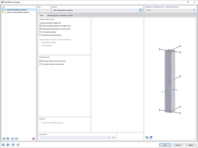
Należy upewnić się, że zdefiniowanie długości efektywnych w aluminiowym module dodatkowym jest warunkiem niezbędnym do przeprowadzenia analizy stateczności. W tym celu w oknie dialogowym należy zdefiniować podpory węzłowe i współczynniki długości efektywnej. Czy chcesz przejrzyście udokumentować podpory węzłowe i wynikające z nich segmenty wraz z powiązanym współczynnikiem długości efektywnej? W celu sprawdzenia wprowadzonych danych najlepiej jest użyć prezentacji graficznej w oknie roboczym programu RFEM/RSTAB. Oznacza to, że możesz zrozumieć projekt w dowolnym momencie i bez większego wysiłku.
- 002463
- Ogólne informacje
- Projektowanie konstrukcji aluminiowych RFEM 6
- Projektowanie konstrukcji aluminiowych RSTAB 9
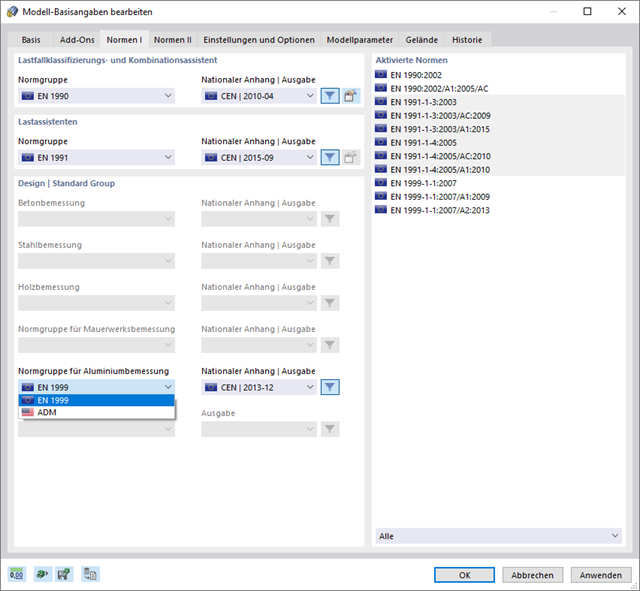
W przypadku obliczeń zgodnie z Eurokodem 9, można znaleźć parametry zintegrowanych załączników krajowych dla następujących krajów:
-
 DIN EN 1999-1-1/NA:2021-03 (Niemcy)
 -
 ÖNORM EN 1999-1-1/NA:2017-11 (Austria)
 -
 SN EN 1999-1-1/NA:2015-01 (Szwajcaria)
 -
 BDS EN 1999-1-1/NA:2014-05 (Bułgaria)
 -
 BS EN 1999-1-1/NA:2014-03 (Wielka Brytania)
 -
 CEN 1999-1-1/2013-12 (Unia Europejska)
 -
 CYS EN 1999-1-1/NA:2019-08 (Cypr)
 -
 CZE EN 1999-1-1/NA:2015-09 (Republika Czeska)
 -
 DS EN 1999-1-1/NA:2019-09 (Dania)
 -
 ELOT EN 1999-1-1/NA:2013-12 (Grecja)
 -
 EVS EN 1999-1-1/NA:2014-01 (Estonia)
 -
 HRN EN 1999-1-1/NA:2015-02 (Chorwacja)
 -
 I S. EN 1999-1-1/NA:2015-01 (Irlandia)
 -
 ILNAS EN 1999-1-1/NA:2013-12 (Luksemburg)
 -
 IST EN 1999-1-1/NA:2014-03 (Islandia)
 -
 LST EN 1999-1-1/NA:2014-03 (Litwa)
 -
 LVS EN 1999-1-1/NA:2015-01 (Łotwa)
 -
 MSZ EN 1999-1-1/NA:2014-04 (Węgry)
 -
 NBN EN 1999-1-1/NA:2014-01 (Belgia)
 -
 NEN EN 1999-1-1/NA:2014-01 (Holandia)
 -
 NF EN 1999-1-1/NA:2016-07 (Francja)
 -
 NP EN 1999-1-1/NA:2014-11 (Portugalia)
 -
 NS EN 1999-1-1/NA:2014-04 (Norwegia)
 -
 PN EN 1999-1-1/NA:2014-05 (Polska)
 -
 SFS EN 1999-1-1/NA:2018-01 (Finlandia)
 -
 SIST EN 1999-1-1/NA:2014-05 (Słowenia)
 -
 SR EN 1999-1-1/NA:2015-01 (Rumunia)
 -
 SS EN 1999-1-1/NA:2013-12 (Szwecja)
 -
 STN EN 1999-1-1/NA:2014-05 (Słowacja)
 -
 TKP EN 1999-1-1/NA:2010-01 (Białoruś)
 -
 UNE EN 1999-1-1/NA:2014-01 (Hiszpania)
 -
 UNI EN 1999-1-1/NA:2014-02 (Włochy)
- 002464
- Wyniki
- Projektowanie konstrukcji aluminiowych RFEM 6
- Projektowanie konstrukcji aluminiowych RSTAB 9
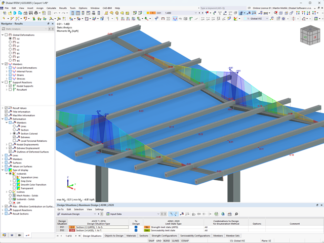
Jak zwykle, wprowadzasz układ i obliczasz siły wewnętrzne w programach RFEM i RSTAB. Masz nieograniczony dostęp do obszernych bibliotek materiałów i przekrojów. Czy wiesz, że za pomocą programu RSECTION można tworzyć przekroje ogólne? Oszczędza to dużo pracy.
Nie bój się'dodatkowych okien i chaosu przy wprowadzaniu danych! Dzieje się tak, ponieważ wymiarowanie aluminium jest w pełni zintegrowane z programami głównymi i automatycznie uwzględnia konstrukcję oraz istniejące wyniki obliczeń. Dalsze dane wejściowe dla obliczeń aluminium, takie jak długości efektywne, redukcje przekroju lub parametry obliczeniowe, można przypisać bezpośrednio do projektowanych obiektów. W wielu miejscach programu najlepiej jest użyć funkcji [Wskaż] do wyboru grafiki - w prosty i efektywny sposób.
- 002465
- Wyniki
- Projektowanie konstrukcji aluminiowych RFEM 6
- Projektowanie konstrukcji aluminiowych RSTAB 9
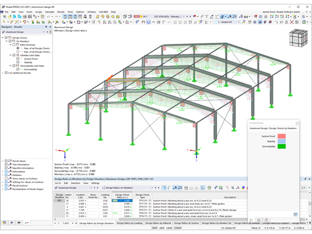
Czy projekt zakończył się sukcesem? Bardzo dobrze, teraz zaczyna się część zrelaksowana. Ponieważ program przedstawia przeprowadzone weryfikacje w formie tabelarycznej. Można wyświetlić szczegółowe informacje o wszystkich wynikach. Dzięki przejrzyście przedstawionym wzorom weryfikacyjnym można bez problemu zrozumieć wyniki. W oprogramowaniu Dlubal nie występuje efekt czarnej skrzynki.
Kontrole są przeprowadzane we wszystkich istotnych punktach prętów i wyświetlane graficznie jako profil wyników. Bardziej szczegółowe grafiki można znaleźć w wynikach wyszukiwania. Obejmuje to na przykład profil naprężenia w przekroju lub kształt drgań własnych.
Wszystkie dane wejściowe i wyniki są częścią protokołu wydruku programu RFEM/RSTAB. Dla poszczególnych obliczeń można wybrać zawartość raportu i żądaną głębokość danych wyjściowych.
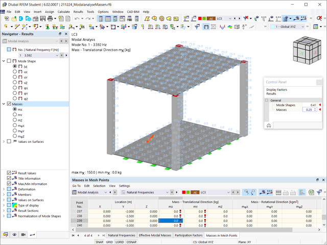
Czy odkryłeś już tabelaryczne i graficzne przedstawianie mas w punktach siatki? Po prawej, jest to również jeden z wyników analizy modalnej w programie RFEM 6. W ten sposób można sprawdzić importowane masy, które zależą od różnych ustawień analizy modalnej. Mogą być one wyświetlane w zakładce Masy w punktach siatki tabeli Wyniki. Tabela zawiera przegląd następujących wyników: Masa - kierunek przesuwny (mX, mY, mZ ), Masa - kierunek obrotowy (mφX, mφY, mφZ ) oraz suma mas. Czy nie byłoby lepiej, gdybyś jak najszybciej przeprowadził ocenę graficzną? Następnie można również wyświetlić graficznie masy w punktach siatki.
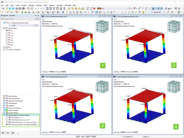
Jak już wiesz, po pomyślnym zakończeniu obliczeń wyniki przypadku obciążenia w Analizie modalnej są wyświetlane w programie. Die erste Eigenform ist für Sie also sofort grafisch oder animiert zu sehen. Dabei können Sie die Darstellung der Eigenformnormierung komfortabel anpassen. Erledigen Sie das am besten direkt im Ergebnisnavigator, wo Sie zur Visualisierung der Eigenformen eine von vier Optionen auswählen:
- Wert des Eigenformvektors uj auf 1 skalieren (berücksichtigt nur die Translationskomponenten)
- Auswahl der maximalen Translationskomponente des Eigenvektors und Einstellung auf 1
- Betrachtung der gesamten Eigenform (inklusive der Rotationskomponenten), Auswahl des Maximums und Einstellung auf 1
- Setzen der modalen Massen mi für jeden Eigenwert auf 1 kg
Ausführlichere Erläuterungen der Normierung der Eigenformen finden Sie hier: Instrukcja online .
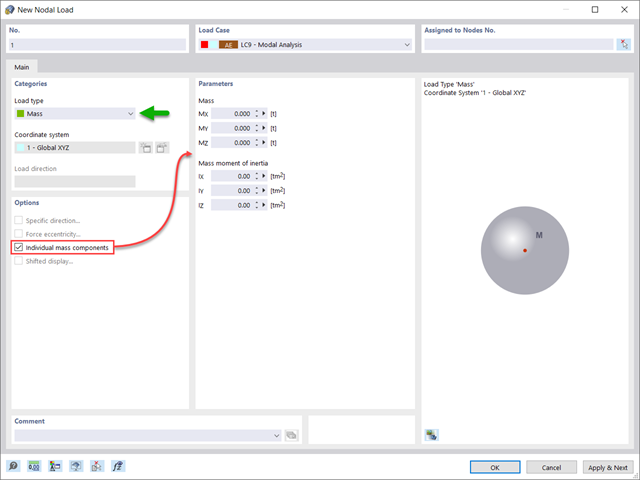
Czy oprócz obciążeń statycznych chcesz uwzględnić również inne obciążenia jako masy? Program umożliwia to dla obciążeń węzłowych, prętowych, liniowych i powierzchniowych. W tym celu podczas definiowania obciążenia należy wybrać typ Obciążenie masą. Dla takich obciążeń należy zdefiniować masę lub składowe masy w kierunkach X, Y i Z. W przypadku mas węzłowych można dodatkowo zdefiniować momenty bezwładności X, Y i Z w celu modelowania bardziej złożonych punktów mas.
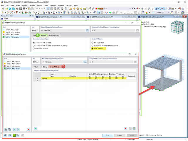
Często zachodzi potrzeba pominięcia mas. Dzieje się tak zwłaszcza w przypadku, gdy wyniki analizy modalnej mają być wykorzystane do analizy sejsmicznej. W tym celu wymagane jest 90% efektywnej masy modalnej w każdym kierunku. Pozwala to na pominięcie masy we wszystkich utwierdzonych podporach węzłowych i liniowych. Program automatycznie dezaktywuje powiązane masy.
Obiekty, których masy mają zostać pominięte w analizie modalnej, można również wybrać ręcznie. Dla lepszego widoku pokazaliśmy to ostatnie na rysunku. W wyniku wyboru przez użytkownika obiektów masowych wraz z skojarzonymi z nimi składowymi masowymi można pominąć masy.
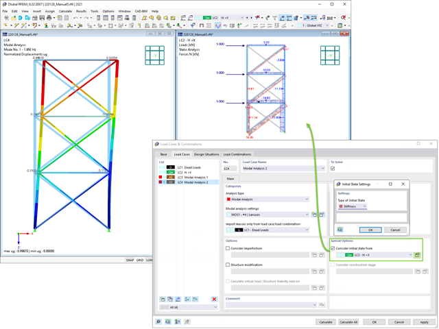
Podczas definiowania danych wejściowych dla przypadku obciążenia analizy modalnej można uwzględnić przypadek obciążenia, którego sztywności reprezentują początkową pozycję analizy modalnej. Jak to zrobić? Jak pokazano na rysunku, należy wybrać opcję "Uwzględnij stan początkowy z". Teraz otwórz okno dialogowe "Ustawienia stanu początkowego" i zdefiniuj typ Sztywność jako stan początkowy. W tym przypadku obciążenia, który jest stanem początkowym branym pod uwagę, można uwzględnić sztywność układu konstrukcyjnego, gdy pręty rozciągane ulegają uszkodzeniu. Celem tego wszystkiego: Sztywność z tego przypadku obciążenia jest uwzględniana w analizie modalnej. W ten sposób uzyskuje się wyraźnie elastyczny system.
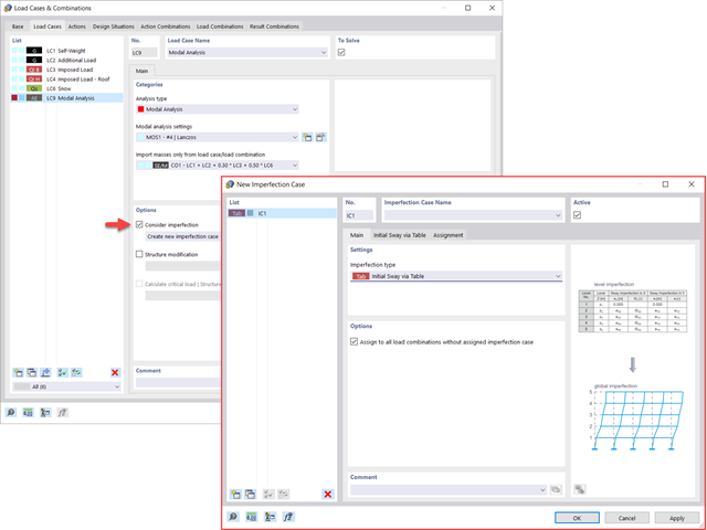
Widać to już na obrazku: Imperfekcje można również uwzględnić podczas definiowania przypadku obciążenia w analizie modalnej. Typy imperfekcji, które mogą być stosowane w analizie modalnej, to obciążenia hipotetyczne z przypadku obciążenia, początkowe przemieszczenie w tabeli, odkształcenie statyczne, postać wyboczeniowa, postać dynamiczna oraz grupa przypadków imperfekcji.
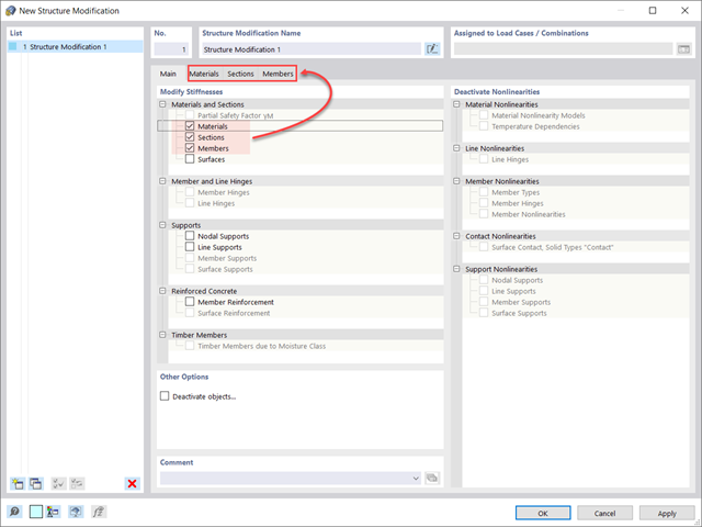
Czy wiecie, że...? W przypadkach obciążeń typu Analiza modalna można z łatwością wprowadzać zmiany konstrukcyjne. Pozwala to na przykład na indywidualne dostosowanie sztywności materiałów, przekrojów, prętów, powierzchni, przegubów i podpór. W przypadku niektórych rozszerzeń można również modyfikować sztywności. Po wybraniu obiektów ich właściwości sztywności są dostosowywane do typu obiektu. W ten sposób można je zdefiniować w osobnych zakładkach.
Czy chcesz przeanalizować uszkodzenie obiektu (na przykład słupa) w analizie modalnej? Jest to również możliwe bez żadnych problemów. Wystarczy przejść do okna Modyfikacja konstrukcji i dezaktywować odpowiednie obiekty.
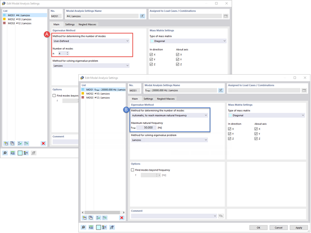
Twoim celem jest określenie liczby postaci drgań własnych? Program oferuje dwie metody. Z jednej strony, można ręcznie zdefiniować liczbę najmniejszych kształtów drgań, które mają zostać obliczone. W tym przypadku liczba dostępnych kształtów postaci zależy od stopni swobody (tzn. liczby punktów mas swobodnych pomnożonych przez liczbę kierunków, w których działają masy). Jest to jednak ograniczone do 9999. Z drugiej strony, maksymalną częstotliwość drgań własnych można ustawić w taki sposób, w jaki program określił kształty automatycznie, aż do osiągnięcia zadanej częstotliwości drgań własnych.
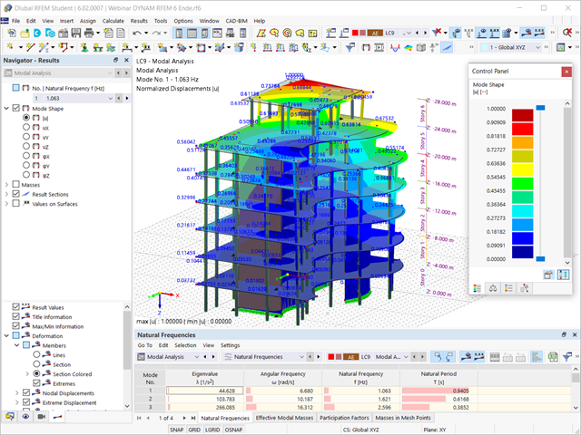
Czy obliczenia się zakończyły? Wyniki analizy modalnej są wówczas dostępne zarówno w formie graficznej, jak i tabelarycznej. Wyświetl tabele wyników dla przypadku obciążenia lub przypadków obciążeń analizy modalnej. Dzięki temu na pierwszy rzut oka można zobaczyć wartości własne, częstotliwości kątowe, częstotliwości i okresy drgań własnych konstrukcji. W przejrzysty sposób wyświetlane są również efektywne masy modalne, modalne współczynniki masy i współczynniki udziału.
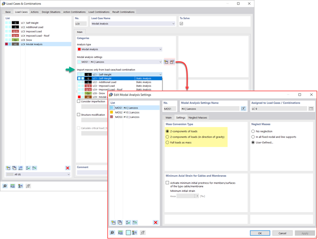
Dostępnych jest kilka opcji definiowania mas dla analizy modalnej. Masy od ciężaru własnego są uwzględniane automatycznie, natomiast obciążenia i masy można uwzględnić bezpośrednio w przypadku obciążenia typu analiza modalna. Potrzebujesz więcej opcji? Należy wybrać, czy obciążenia pełne mają być uwzględniane jako masy, składowe obciążenia w globalnym kierunku Z, czy tylko składowe obciążenia w kierunku siły ciężkości.
Program oferuje dodatkową lub alternatywną opcję importu mas: Ręczna definicja kombinacji obciążeń, począwszy od których masy są uwzględniane w analizie modalnej. Wybrałeś normę obliczeniową? Następnie można utworzyć sytuację obliczeniową typu Kombinacja mas sejsmicznych. W ten sposób program automatycznie oblicza sytuację masową dla analizy modalnej zgodnie z preferowaną normą obliczeniową. Innymi słowy: Program tworzy kombinację obciążeń na podstawie współczynników kombinacji wstępnie ustawionych dla wybranej normy. Zawiera on masy użyte do analizy modalnej.